கணினி தரவமைப்புகளும் செயல்முறைகளும்

கணினி தரவமைப்புகளும் செயல்முறைகளும்
Tamil Translation of “Practical Algorithms and Data Structures”
தமிழாக்கம் வெளியீடு : 2022, எழில் மொழி அறக்கட்டளை
கணினி தரவமைப்புகளும் செயல்முறைகளும்
இந்த நூல் "Practical Algorithms and Data Structures" என்ற ஆங்கில புத்தகத்தின் தமிழாக்கமாகும். இந்த நூலில் தமிழ் கலைச்சொற்கள் 'ரூபி நண்பன்', 'எழில் - தமிழில் நிரல் எழுது' போன்ற நூல்களின் நடையில் கையாளப்படும் என்று எண்ணுகின்றோம். Practical Algorithms and Data Structures என்ற நூல் "Problem Solving with Algorithms and Data Structures Using Python," என்ற, பகிர்வு உரிமத்தின் கீழ் வெளியிடப்பட்ட, நூலைத் தழுவி எழுதப்பட்டது. காண்க: http://www.openbookproject.net/books/pythonds/
இந்த நூல் பிராட்பீல்டு கணினி கல்லூரியினால், பொது உரிமத்தின் கீழ், வெளியிடப்பட்டது: https://bradfieldcs.com/algos

Problem Solving with Algorithms and Data Structures using Python by Bradley N. Miller, David L. Ranum is licensed under a Creative Commons Attribution-NonCommercial-ShareAlike 4.0 International License. தமிழ் தரவமைப்புகளின் சொல்லாடல் சுட்டி
அச்சமைப்பு: Jan 4, 2022, Ezhil Language Foundation : ezhillang@gmail.com | Revision #4
தமிழாக்கம்: விமலன் குமரகுலசிங்கம், முத்தையா அண்ணாமலை
ஆசிரியர் திருத்தம்: பரதன் தியாகலிங்கம், குப்பன் சர்க்கரை, மலர் கதிரேசன், சுந்தரப்பன் கதிரேசன்
வெளியீடப்பட்ட ஊர்: வட கலிபோர்னியா - சான் பிரான்சிஸ்கோ விரிகுடா பகுதி, அமெரிக்கா.
அட்டைப்படம்: © 2008, முத்து அண்ணாமலை; இடம்: யோசமிட்டி தேசிய பூங்கா, அமெரிக்கா.
பொருளடக்கம்
கணினி தரவமைப்புகளும் செயல்முறைகளும் 1
கணினி தரவமைப்புகளும் செயல்முறைகளும் 2
1. நடைமுறையில் கணினி தரவமைப்புகளும் செயல்முறைகளும் - Practical Algorithms and Data Structures 7
1.1 மேற்பார்வை (The Big Picture) 9
1.2 கணிமை சிக்கலளவு (Big O Notation) 14
1.3 சொல்புதிர் எடுத்துக்காட்டு - An Anagram Detection Example 19
Solution 1: Checking Off - விடைமுறை 1 எழுத்துக்களை குறித்தல் 19
Solution 2: Sort and Compare - விடைமுறை 2 வரிசைப்படுத்தி ஒப்பிடுதல் 20
Solution 3: Brute Force - விடைமுறை 3 முழுத்தேடல் 21
Solution 4: Count and Compare - விடைமுறை 4 எண்ணி ஒப்பிடுதல் 21
1.4 பைத்தன் தரவு வகையின் கணிமைச்சிக்கலளவு - Performance of Python Types 24
சுட்டுவரிசையாக்கம் & ஒதுக்கீடுதல் (Indexing & Assigning) 24
சேர்த்தல் & இணைத்தல் (Appending & Concatenating) 24
மேலெடுத்தல்,முறைமாற்றல் & நீக்குதல் (Popping, Shifting & Deleting) 25
மீள்செயல் & நகலெடுத்தல் ( Iterating & Copying ) 27
சராசரி நிலை(The “Average Case”) 27
2.1 அடுக்குகள் ஓரு அறிமுகம் 30
உருவற்ற தகவல் தரவமைப்பு - Stack Abstract Data Type 32
2.2 அடுக்குகளின் செயற்பாடு - A Stack Implementation 34
2.3 சமமான அடைப்புக்குறிகள் - Balanced Parentheses 37
சமமான அடைப்புக்குறிகள் பொதுவான தீர்வு - Balanced Symbols: A General Case 39
2.4 எண்களை நிலைமாற்றல் - Converting Number Bases 42
2.5 Infix, Prefix and Postfix Expressions - நடுஒட்டு, முன்/பின் ஒட்டு சூத்திரங்கள் 46
Conversion of Infix Expressions to Prefix and Postfix - குறிமுறை மாற்றம் 48
General Infix-to-Postfix Conversion - பொதுவான சூத்திரங்கள் குறிமுறை மாற்றம் 49
Postfix Evaluation - பின்னொட்டு கணித்தல் 52
3.1 வரிசைகள் அறிமுகம் - Introduction to Queues 56
3.2 வரிசை தகவல் தரவமைப்பு - The Queue Abstract Data Type 57
3.3 A Queue Implementation- வரிசை செயற்படுத்தல் 58
3.4 அவிச்ச கிழங்கு விளையாட்டு ஒத்திகை - Simulating Hot Potato 58
4.1 இருதிசை வரிசை அறிமுகம் - Introduction to Deques 63
4.1.1 இருதிசை வரிசை தகவல்தரவமைப்பு - The Deque Abstract Data Type 63
4.2 இருதிசை வரிசை செயற்படுத்தல் - A Deque Implementation 65
4.3 விகடகவி பரிசோதனை - Palindrome Checker 67
5.1 பட்டியல் அறிமுகம் - Introduction to Lists 70
5.1.1 சீரிலா பட்டியல் உருவற்ற தரவமைப்பு அம்சங்கள் - The Unordered List Abstract Data Type 70
5.2 சீரான பட்டியல் - The Ordered List 71
5.2.1 சீரிலா பட்டியல் - Implementing an Unordered List 72
சீரற்ற பட்டியல் வகை - The Unordered List Class 73
5.3 சீரான பட்டியல் - Implementing an Ordered List 80
5.4 தொடர்பட்டியல் திறணாய்வு - Analysis of Linked Lists 82
6.1 அடுக்கு நிரல்படுத்தல் அறிமுகம் - Introduction to Recursion 85
6.2 எண் பட்டியலின் கூட்டுமதிப்பு - Calculating the Sum of a List of Numbers 86
6.3 மூன்று விதிகள் - The Three Laws of Recursion 90
6.4 எண்களை குறிப்பிட்ட தளத்திற்கு மாற்றுவது - Converting an Integer to Any Base 91
6.5 ஹனோய் கோபுரங்கள் - Tower of Hanoi 94
6.6 நிகழ்வு நிரலாக்கம் - Dynamic Programming 97
6.7 அடுக்கு நிரலாக்கத்தை செயற்படுத்தல் - Implementing Recursion 103
7.2 வரிசைபடுத்தப்பட்ட தேடல் - Sequential Search 107
தொடர்ச்சியான தேடலின் திறனாய்வு - Analysis of Sequential Search 108
7.3 இரும நிலை தேடல் - The Binary Search 110
Analysis of Binary Search - இரும நிலைத்தேடல் திறணாய்வு 111
7.4 Hashing - எண்ணம் அடைவாக்கம் 113
Hash Functions - அடைவாக்க சார்புகள் 114
Collision Resolution - அடைவாக்கத்தில் தனித்துவம் காத்தல் 117
Analysis of Hashing - அடைவாக்கம் திறணாய்வு 120
8.1 Introduction to Trees - இருகிளை மரம் தரவமைப்பு அறிமுகம் 122
Examples of trees - இருகிளை மரம் உதாரணங்கள் 122
8.2 மரம் தரவமைப்பின் பிரதிநிதித்துவம் - Representing a Tree 129
உச்சிகள் மற்றும் குறிப்புக்களின் பிரதிநிதித்துவம்(Nodes and references representation) 129
பட்டியல்கள் பட்டியலின் பிரதிநிதித்துவம் (List of lists representation) 132
விவரணையாக்கப் பிரதிநிதித்துவம் (Map-based representation) 135
8.3 பகுப்பாய்வு மரங்கள் - Parse Trees 137
8.4 மரம் தரவமைப்பு பயணித்தல் - Tree Traversals 146
8.5 Priority Queues with Binary Heaps 149
(கட்டமைப்பு சொத்து) The Structure Property 149
குவியல் வரிசை அம்சம் - The Heap Order Property 150
குவியல் செயல்பாடுகள் - Heap Operations 151
8.6 இருகிளை தேடல்மரம் - Binary Search Trees 159
செயற்படுத்தல் - Implementation 159
8.7 AVL மரம் தரவமைப்பு - AVL Trees 172
செயல்படுத்தல் - Implementation 174
9.1 அறிமுகம் - Introduction to Graphs 184
The Graph Abstract Data Type 186
9.2 முனை ஓரம் தரவமைப்பின் குறிமுறை - Representing a Graph 187
அண்மைய அச்சு வார்ப்புரு (The Adjacency Matrix) 187
அண்மைய பட்டியல் (The Adjacency List) 188
பொருள் நோக்கு நிரலாக்கம் - An Object-Oriented Approach 189
நேரடியாக தொடர்புறு அணியைப் பயன்படுத்துதல் (Using Dictionaries Directly) 192
9.3 சொல் ஏணிகள் விளையாட்டு - Word Ladders 193
Building the Word Ladder Graph 193
Implementing breadth first search 196
Breadth First Search Analysis 200
Building the Knight’s Tour Graph 202
Implementing Knight’s Tour 204
9.5 General Depth First Search 212
9.7 Shortest Path with Dijkstra’s Algorithm 220
Analysis of Dijkstra’s Algorithm 226
9.8 Strongly Connected Components 227
9.9 Prim’s Spanning Tree Algorithm 232
இணைப்பு - அ : அடிப்படடை தரவுவகைகள் - Fundamental Datatypes 241
Glossary - கலைச்சொற்கள் அகராதி 242
1. நடைமுறையில் கணினி தரவமைப்புகளும் செயல்முறைகளும் - Practical Algorithms and Data Structures
இந்த நூல் கணினியில் துறையின் முக்கியமான தகவல் தரவமைப்புகள் மற்றும் செயல்முறைகள் பற்றியும் நடைமுறையில் பயன்படுவதாகவும் ,நகைச்சுவையாகவும் (முடிந்தளவு) இருப்பதற்கு முயல்கிறோம்.
நிறைய பொறியாளர்களும் நிரலர்களும் “நடைமுறை கணினி தரவமைப்புகள்” என்பதை ஒரு எதிர்மறையானதாக நினைக்கின்றனர் 😞 ஆகையால் இந்த நூலை எளிதாகவும், சுருக்கமாகவும் வைத்துள்ளோம்.1 இதன்படி நடைமுறைக்கு உதவுமாறு கணினி நிரல்களை பைத்தன் மொழியில் வெளியிட்டுள்ளோம்.
சுவாரசியமான தலைப்புகளில் (graph traversal) முனை-ஓரம் பயணித்தல் , (dynamic programming) இயங்குநேர நிரலாக்கல் ஆகியவற்றிற்கு விரிவாக பாடங்களை இணைத்துள்ளோம். இதன் காரணம் என்னவெனில்தினசரி செயல்பாடுகளில் முனை-ஓர பயனித்தல்களை அடிக்கடி பயன்படுத்தியும் வரிசைபடுத்தும் செயல்பாடுகள் (quicksort) போன்றவற்றினை விட அதிகமாக உள்ளதாகும் .. இங்கு இணைக்கப்படாத செயல்முறைகளும் எங்களுக்கு பரிட்சயமானது - எனினும் அவைகள் அங்கங்கு இணைக்கப்படுள்ளன.
இந்த நூல் Brad Miller, David Ranum அவர்களது நூலான "Problem Solving with Algorithms and Data Structures Using Python," என்ற மூலத்தில் இருந்து உருவாக்கப்பட்டது; இந்த நூல் பொது உரிமத்தின் கீழ் (Creative Commons) வெளியிடப்பட்டதால் இது சாத்தியமாயிற்று. மூல நூலை எங்களது Bradfield கல்லூரி பாட திட்டத்தின் வழி பெற்ற அனுபவங்களின் வாயிலாக மாற்றி எழுதுகிறோம். எங்களது நூல் மேலும் அதே பொது உரிமத்தின் கீழ் வெளியாகிறது - இதனை மேம்படுத்த இணை வேண்குகோள் (pull request) அனுப்பலாம்.
தமிழாக்கம் குறிப்பு: இந்த நூலின் மூல தமிழாக்கம் பொது உரிமத்தின் கீழ் வெளியாகிறது - இதனை மேம்படுத்த இணை வேண்குகோள் (pull request) அனுப்பலாம். எங்களது மற்ற நூல்களான "ரூபி நண்பன்," என்பதை இங்கும், எழில் மொழி அறிமுக நூல் என்பதை இங்கும் காணலாம்
1.0 Analysis - அல்கொரிதம் திறனாய்வு1.1 மேற்பார்வை (The Big Picture)
ஒரு கணினி நிரலை மற்றொன்றை விட சிறந்ததாக ஆக்குவது எப்படி?
இதற்கு நீங்களே பதில் சொல்ல சிறிது நேரம் ஒதுக்குங்கள்🙂. ஒரே பிரச்சனையை தீர்க்கும் இரண்டு செயல்திட்டங்கள் உங்களுக்கு வழங்கப்பட்டால், அவற்றுக்கிடையே நீங்கள் எப்படி முடிவு செய்வீர்கள்?
உண்மை என்னவென்றால், அவைகளுக்காக பல சரியான அளவுகோள்ள் உள்ளன, அவை பெரும்பாலும் சிக்கலானவையாக உள்ளன.
எங்கள் செயல்திட்டம் சரியாக இருக்க வேண்டும் என்று நாங்கள் பொதுவாக விரும்புகிறோம். வேறு சொற்களில் கூறுவதானால், அந்த செயல்திட்டத்தின் வெளியீடு எங்கள் எதிர்பார்ப்புகளுடன் பொருந்த வேண்டும். துரதிர்ஷ்டவசமாக, சரியானது எப்போதும் தெளிவாக இருப்பதில்லை. உதாரணமாக, உங்கள் தேடல் வினவலுக்கான "சரியான" முதல் 10 தேடல் முடிவுகளை கூகுள் வழங்குவதன் அர்த்தம் என்ன?
நல்ல மென்பொருள் பொறியாளர்கள் பெரும்பாலும் தங்கள் நிரல்கள் வாசிக்க கூடியதானதாக , மீண்டும் பயன்படுத்தக்கூடிய, நேர்த்தியான அல்லது பரிசோதிக்கக்கூடியதாக இருக்க விரும்புகிறார்கள். இவை போற்றத்தக்க இலக்குகள், ஆனால் அவை அனைத்தையும் ஒரே நேரத்தில் அடைய முடியாமல் போகலாம். "நேர்த்தியானது" எப்படி இருக்கிறது என்பது முற்றிலும் தெளிவாக இல்லை, மேலும் கணித ரீதியாக எங்களால் நிச்சயமாக அதை வடிவமைக்க முடியவில்லை, எனவே கணினி விஞ்ஞானிகள் நிரல்களின் இந்த அம்சங்களை அதிகம் கருத்தில் கொள்ளவில்லை 🤷
கணிப்பொறி விஞ்ஞானிகள் கணித மாதிரியை உருவாக்கும் போது விரும்பும் இரண்டு காரணிகள், ஒரு நிரல் இயங்க எவ்வளவு நேரம் எடுக்கும், எவ்வளவு இடத்தை (பொதுவாக, நினைவகம்) பயன்படுத்திகொள்ளும் என்பதாகும் . நாங்கள் இந்த நேரத்தையும் இடத்தின் செயல்திறனையும் பயன்படுத்துவதோடு , மேலும் அவைகளுக்கான வழிமுறைகளே எங்கள் ஆய்வின் மையமாக இருக்கும்.
கருத்தில் கொள்ளவேண்டியவற்றிற்கு எதிராக நாம் இதை பரிமாற்றம் செய்ய வேண்டியிருக்கலாம்: வழிமுறை A விரைவானதாக இருக்கலாம் ஆனால் வழிமுறை B. ஐ விட அதிக நினைவகத்தைப் பயன்படுத்தலாம். அவை இரண்டும் வழிமுறை C ஐ விட குறைவான நேர்த்தியுடன் இருக்கலாம். நாங்கள் நேரத்திலும் இடத்திலும் கவனம் செலுத்துவோம், ஏனென்றால் அவை சுவாரஸ்யமானவை, அளவிடக்கூடியவை, ஆனால் தயவுசெய்து அவை எப்போதும் மிக முக்கியமான காரணிகள் என்று நினைத்து விடாதீர்கள் உண்மையிலேயே சரியான பதில்: "அவை சார்ந்தவை அல்லது தங்கியுள்ளவை".
"இது சார்ந்தவை" என்பதன் மற்றொரு அம்சம், நாம் நேரம் அல்லது இடைவெளியில் மட்டும் கவனம் செலுத்தினால் கூட, எந்த நிரல் இயங்குகின்றது என்பதிலும் தங்கும். ஒரு நிரலின் உள்ளீடுகளுக்கும் அதன் இயங்கும் நேரம் அல்லது இடம் பயன்பாட்டிற்கும் இடையே எப்போதும் ஒரு உறவு இருக்கும். உதாரணமாக, நீங்கள் பல பெரிய கோப்புகளை grep தேடல் செய்வதற்காக எடுக்கும் நேரம் குறைவானது . சிறிய கோப்புகளை நீங்கள் கிரெப் செய்தால் எடுக்கும் நேரத்தைவிட அதிகமானது . உள்ளீடுகளுக்கும் நடத்தைக்கும் இடையிலான இந்த உறவு எங்கள் பகுப்பாய்வின் ஒரு முக்கிய பகுதியாக இருக்கும்.
இதைத் தாண்டி, உங்கள் நிரல் பயன்படுத்தும் சரியான நேரமும் இடமும் பல காரணிகளைப் பொறுத்தது. உங்களால் குறைந்தது மூன்று காரணிகளைப் பற்றி யோசிக்க முடியுமா?
அவற்றுள் சில பின்வருமாறு:
- ஒவ்வொரு அறிவுறுத்தலையும் செயல்படுத்த உங்கள் கணினி எவ்வளவு நேரம் எடுக்கும்
- உங்கள் கணினியின் "Instruction Set Architecture", உதாரணமாக ARM அல்லது Intel x86
- நிரல் உங்கள் இயந்திரத்தின் எத்தனை cores பயன்படுத்துகிறது
- உங்கள் நிரல் எந்த மொழியில் எழுதப்பட்டுள்ளது
- உங்கள் இயக்க முறைமை செயல்முறைகளை திட்டமிடுவதற்கு எவ்வாறு தேர்வு செய்கிறது
- அதே நேரத்தில் வேறு என்ன நிரல்கள் இயங்குகின்றன
… மேலும் பல உள்ளன.
இவை அனைத்தும் நடைமுறையில் முக்கியமானவை, ஆனால் ஒரு வழிமுறை பொதுவாக மற்றொன்றை விட சிறந்ததா அல்லது மோசமானதா என்ற முக்கிய கேள்விக்கு யாரும் தீர்வு காணவில்லை. சில நேரங்களில் நாம் பொதுவாக கேட்க விரும்புகிறோம்:, IBM 704 க்காக Fortran ஒரு நிரல் எழுதப்பட்டிருந்தாலும் அல்லது பளபளப்பான புதிய மேக்புக்கில் இயங்கும் பைத்தானில் இருந்தாலும், அது மரத்தை விட நேரம் மற்றும்/அல்லது இடத்தை பயன்படுத்துவதில் திறமையாக இருக்குமா? இது குறைந்த இடத்தை பயன்படுத்துமா? இது வழிமுறை பகுப்பாய்வின் முக்கிய அம்சமாகும்.
வழிமுறை திறனாய்வு என்பது நிரல்களின் சாத்தியமான உள்ளீடுகளுடன் நேரம் மற்றும் இட செயல்திறன் ஆகியவற்றினை ஒப்பிடுவதற்கான ஒரு வழியாகும், ஆனால் மற்ற சூழலைப் பொருட்படுத்தாது .
நிஜ உலகில், சில அலகுகளில் ஒரு நிரல் பயன்படுத்தும் நேரத்தை அளவிடுகிறோம் அது நேரத்தின் சில அலகுகளால் கணக்கிடப்படுகின்றது , அதாவது வினாடிகள். இதேபோல் பைட்டுகள் போன்றவற்றில் பயன்படுத்தப்படும் இடத்தை அளவிடுகிறோம். பகுப்பாய்வில், இது மிகவும் குறிப்பிடத்தக்கதாக இருக்கும். முடிக்க எடுக்கும் நேரத்தை நாம் அளந்தால், இந்த எண் மொழி தேர்வு மற்றும் CPU வேகம் போன்ற விவரங்களை உள்ளடக்கும். நாம் தேடும் பொதுத்தன்மையுடன் பேசுவதற்கு எங்களுக்கு புதிய மாதிரிகள் மற்றும் சொல்லகராதி தேவைப்படும்.
இந்த யோசனையை ஒரு எடுத்துக்காட்டுடன் ஆராய்வோம்.
முதல் n எண்களின் தொகையை நான் கணக்கிட விரும்பினேன் என்றால் , இதற்கு எவ்வளவு நேரம் ஆகும் என்று நான் யோசித்துக் கொண்டிருக்கிறேன். முதலில், கணக்கீடு செய்ய ஒரு எளிய வழிமுறையை நீங்கள் யோசிக்க முடியுமா? இது ஒரு செயலுருபு n கொண்ட ஒரு செயல்பாடாக இருக்க வேண்டும், மேலும் முதல் n எண்களின் கூட்டுத்தொகையை அளிக்கும். நீங்கள் மேலதிகமாக எதையும் செய்யத் தேவையில்லை, ஆனால் தயவுசெய்து ஒரு வழிமுறையை எழுத நேரம் ஒதுக்கி, சிறிய அல்லது பெரிய உள்ளீடுகளில் இயங்க எவ்வளவு நேரம் ஆகும் என்று சிந்தியுங்கள்.
இங்கே ஒரு எளிய பைதான் தீர்வு,
def sum_to_n(n): total = 0 for i in range(n + 1): total += i return total |
ஒரு பெரிய n கொடுக்கப்பட்டால் sum_to_n ஐ இயக்க அதிக நேரம் எடுக்குமா? “உள்ளுணர்வாக, பதில் ஆம் என்று தோன்றுகிறது, ஏனெனில் அது இன்னும் பல முறை சுழலும்.
Sum_to_n ஒவ்வொரு முறையும் ஒரே உள்ளீட்டைக் கொண்டு இயக்க அதே நேரத்தை எடுக்குமா? உள்ளுணர்வாக பதில் ஆம் என்று தோன்றுகிறது, ஏனெனில் அதே அறிவுறுத்தல்கள் செயல்படுத்தப்படுகின்றன.
இப்போது சில சுயாதீன நிரல் வரிகளை சேர்ப்போம்:
import time def sum_to_n(n): # record start time start = time.time() # run the function's code total = 0 for i in range(n + 1): total += i # record end time end = time.time() return total, end - start |
நான் இதை n = 1000000 (1 மில்லியன்) உடன் இயக்கினேன் என்று சொல்லலாம், அது 0.11 வினாடிகள் எடுத்தது. நான் இன்னும் ஐந்து முறை இயக்கினால் நீங்கள் என்ன எதிர்பார்க்கிறீர்கள்?
>>> output_template = '{}({}) = {:15d} ({:8.7f} seconds)'
>>> for _ in range(5):
... print(output_template.format('sum_to_n', 1000000, *sum_to_n(1000000)))
sum_to_n(1000000) = 500000500000 (0.1209280 seconds)
sum_to_n(1000000) = 500000500000 (0.1107872 seconds)
sum_to_n(1000000) = 500000500000 (0.1187370 seconds)
sum_to_n(1000000) = 500000500000 (0.1210580 seconds)
sum_to_n(1000000) = 500000500000 (0.1230309 seconds)
சுவாரஸ்யமாக, ஒவ்வொரு முறையும் எனது கணினி மற்றும் பைதான் மெய்நிகர் இயந்திரத்தின் சற்று மாறுபட்ட நிலை காரணமாக, ஒவ்வொரு அழைப்பிலும் சிறிது வித்தியாசமான நேரம் எடுக்கும். நாம் பொதுவாக இதுபோன்ற சிறியதும், சீரற்றதுமான வேறுபாடுகளை புறக்கணிக்க விரும்புகிறோம்.
இப்போது, 1 மில்லியன், 2 மில்லியன், 3 மில்லியன், 9 மில்லியன் வரை பல்வேறு உள்ளீடுகளுடன் மீண்டும் இயங்கினால் என்ன செய்வது? நீங்கள் எதைப் பார்க்க எதிர்பார்க்கிறீர்கள்?
>>> for i in range(1, 10):
... print(output_template.format('sum_to_n', i * 1000000, *sum_to_n(i * 1000000)))
sum_to_n(1000000) = 500000500000 (0.1198549 seconds)
sum_to_n(2000000) = 2000001000000 (0.2401729 seconds)
sum_to_n(3000000) = 4500001500000 (0.3838110 seconds)
sum_to_n(4000000) = 8000002000000 (0.4790699 seconds)
sum_to_n(5000000) = 12500002500000 (0.6189690 seconds)
sum_to_n(6000000) = 18000003000000 (0.6952291 seconds)
sum_to_n(7000000) = 24500003500000 (0.8431778 seconds)
sum_to_n(8000000) = 32000004000000 (0.9679160 seconds)
sum_to_n(9000000) = 40500004500000 (1.0458572 seconds)
n க்கும் நேரத்திற்கும் இடையே உள்ள பொதுவான உறவை நீங்கள் பார்க்கிறீர்களா? நீங்கள் எதிர்பார்த்தது இதுதானா? நீங்கள் x அச்சில் n இன் மதிப்புகளையும், y அச்சில் செயல்படுத்தும் நேரத்தையும் வரைந்தால் உறவு எப்படி இருக்கும்?

எங்கள் எளிய உத்தி மிகவும் திறமையானது அல்ல என்று மாறிவிடும். உண்மையில் ஒரு குறுகிய சூத்திரம் உள்ளது, அது எந்த வளையமும் இல்லாமல் நம் கேள்விக்கான பதிலைத் தரும். அது என்ன என்பதை உங்களால் தீர்மானிக்க முடியுமா (அல்லது ஒருவேளை நினைவில் இருக்கலாம்)? இங்கே ஒரு குறிப்பு உள்ளது: 1 மற்றும் 6, 2 மற்றும் 5, மற்றும் 3 மற்றும் 4 ஆகியவற்றை ஒன்றாக தொகுத்து 1 முதல் 6 வரையிலான எண்களை தொகுக்க முயற்சிக்கவும், ஒவ்வொன்றும் மொத்தம் 7 என மூன்று ஜோடிகள் இருப்பதைக் கவனியுங்கள்.
கணித ரீதியாக, சூத்திரம்:

இந்த சூத்திரம் உங்களுக்கு சரியாக புரியவில்லை என்றால், இந்த காட்சி விளக்கங்களில் ஒன்றை ஆராய சிறிது நேரம் ஒதுக்குங்கள். இதை எப்படி பைதான் செயல்பாடாக, மீண்டும் நமது நேர நிரலாக்கத்துடன் செயல்படுத்துவது?
def arithmetic_sum(n):
start = time.time()
total = n * (n + 1) // 2
end = time.time()
return total, end - start
What do you expect to see if we run this with a range of inputs as we did with sum_to_n?
>>> for i in range(1, 10):
... print(output_template.format('arithmetic_sum', i * 1000000, *arithmetic_sum(i * 1000000)))
n க்கும் நேரத்திற்கும் இடையே உள்ள பொதுவான தொடர்பினை நீங்கள் பார்க்கிறீர்களா? நீங்கள் எதிர்பார்த்தது இதுதானா? நீங்கள் x- அச்சில் n இன் மதிப்புகள் மற்றும் y- அச்சில் செயல்படுத்தும் நேரத்தை அமைத்தால் தொடர்பு எப்படி இருக்கும்?
arithmetic_sum(1000000) = 500000500000 (0.0000021 seconds)
arithmetic_sum(2000000) = 2000001000000 (0.0000029 seconds)
arithmetic_sum(3000000) = 4500001500000 (0.0000019 seconds)
arithmetic_sum(4000000) = 8000002000000 (0.0000019 seconds)
arithmetic_sum(5000000) = 12500002500000 (0.0000031 seconds)
arithmetic_sum(6000000) = 18000003000000 (0.0000021 seconds)
arithmetic_sum(7000000) = 24500003500000 (0.0000021 seconds)
arithmetic_sum(8000000) = 32000004000000 (0.0000029 seconds)
arithmetic_sum(9000000) = 40500004500000 (0.0000019 seconds)
sum_to_n இல் செய்தது போல், உள்ளீடுகளின் வரம்பில் இதை இயக்கினால் என்ன எதிர்பார்க்கிறீர்கள்?

நமது y அச்சு இப்போது மைக்ரோ வினாடிகளில் குறிக்கப்பட்டுள்ளது,அவை ஒரு வினாடிக்கு மில்லியன் ஆகும் . செயல்படுத்தும் நேரம் உள்ளீட்டின் அளவிலிருந்து பெரும்பாலும் சுயாதீனமாகத் தோன்றுகிறது என்பதையும் கவனிக்கவும்.
நாம் sum_to_n ஐ "நேரியல்" அல்லது O (n) என்றும், arithmetic_sum " ஆனது மாறிலி" அல்லது O (1) என்றும் விவரிக்கிறோம். இது ஏன் என்று நீங்கள் பார்க்க ஆரம்பிக்கலாம். இந்த செயல்பாடுகளைச் செயல்படுத்துவதற்கு சரியான நேரங்களைப் பொருட்படுத்தாமல், ஒரு பொதுவான போக்கை நாம் காணலாம், sum_to_n க்கான செயல்பாட்டு நேரம் n விகிதத்தில் வளரும் போது arithmetic_sum தொடர்ந்தும் மாறிலியாக இருப்பதால், இந்த காரணத்திற்காக arithmetic_sum சிறந்த வழிமுறையாகும்.
பின்வரும் பகுதிகளில் , எங்களுக்கான காரணங்களுக்காக இன்னும் கொஞ்சம் கண்டிப்பைப் பயன்படுத்துவோம், மேலும் நேரமும் அளவீடும் இல்லாமல் இந்த நேரத்தையும் இடப் பண்புகளையும் தீர்மானிப்பதற்கான ஒரு முறையை ஆராய்வோம்.
1.2 கணிமை சிக்கலளவு (Big O Notation)
ஒரு வழிமுறை(Algorithm) என்பது சில பணிகளை செய்து முடிப்பதற்கான தொடர் படிமுறைகளை காட்டிலும் சற்று விரிவானது அல்லது சிறந்தது. பணியினை செய்து முடிப்பதற்கான ஒவ்வொரு படிமுறைகளையும் அந்த பணியை செய்து முடிப்பதற்கான கணிப்பீட்டின் அடிப்படை அலகாக கருத்தின், வழிமுறையின் செயற்பாட்டு நேரம் என்பது சிக்கலை தீர்ப்பதற்கு தேவைப்பட்ட படிமுறைகள் எண்ணிக்கையினால் வெளிப்படுத்தப்படலாம். இதனை கணிமை சிக்கலளவு (computational complexity) என்றும் சொல்லலாம்.
இந்த சுருக்கம் நமக்குத் தேவையானது: எந்தவொரு குறிப்பிட்ட நிரல்(program) அல்லது கணினியிலிருந்து சுயாதீனமாக இருக்கும்போது செயல்பாட்டு நேரத்தின் அடிப்படையில் ஒரு வழிமுறையின் செயல்திறனை இது வகைப்படுத்துகிறது. கடந்த அத்தியாயத்தில் நாங்கள் அறிமுகப்படுத்திய இரண்டு தொகுப்பு(summation) வழிமுறைகளை இப்போது நாம் நெருக்கமாகப் பார்க்கலாம்.
உள்ளுணர்வாக, முதல் வழிமுறை(sum_of_n) இரண்டாவது வழிமுறையை(arithmetic_sum) விட அதிகமாக வேலை செய்வதை நாம் காணலாம்: சில நிரல் படிகள் மீண்டும் மீண்டும் செய்யப்படுகின்றன, மேலும் நாம் n இன் மதிப்பை அதிகரித்தால் நிரல் இன்னும் அதிக நேரம் எடுக்கும். ஆனால் நாம் இன்னும் துல்லியமாக இருக்க வேண்டும்.
Sum_of_n இல் மிகவும் கடினமான அலகு மாறி(variable) ஒதுக்கீடு ஆகும். நாம் ஒதுக்கீடு அறிக்கைகளின்(statements) எண்ணிக்கையை கணக்கிட்டால், வழிமுறையின் செயல்பாட்டு நேரத்தின் சிறந்ததொரு தோராயமான பெறுமானத்தை நாங்கள் பெறுவோம்: ஒரு ஆரம்ப ஒதுக்கீடு அறிக்கை (total = 0) இது ஒரு முறை மட்டுமே செய்யப்படுகிறது, அதனைத் தொடர்ந்து ஒரு நிரலாக்க வளையம் முற்றாக (total += i) n எண்ணிக்கையில் செயற்படுத்தப்படுகின்றது.
இதை நாம் மிகச் சுருக்கமாக செயல்பாடு(function) T என குறிப்பிடலாம், எப்போதென்றால் T(n)=1+n ஆக இருக்கும்போது
செயலுருபு n பெரும்பாலும் "பிரச்சனையின் அளவு" என்று குறிப்பிடப்படுகிறது, எனவே இதை நாம் T(n) அழைக்கலாம். T(n) என்பது n அளவுள்ள பிரச்சனையை தீர்ப்பதற்கு எடுக்கும் நேரமாகும்.இது 1 + n படிமுறைகளினால் குறிப்பிடப்படுகின்றது.
எங்கள் தொகுப்பு செயல்பாடுகளுக்கு, சிக்கலின் அளவைக் கணக்கிடுவற்கு பயன்பட்ட படிமுறைகளின் எண்ணிக்கையைப் பயன்படுத்துவது அர்த்தமுள்ளதாக இருக்கிறது.பின்னர் ,1,000 முழு எண்களின் கூட்டுத்தொகையை கணக்கிடும் பிரச்சனையை விட 100,000 முழு எண்களின் கூட்டுத்தொகையை கணக்கிடும் பிரச்சனை பெரிதென்பதை உதாரணமாக குறிப்பிடலாம்.
மேலுள்ள கூற்றின் அடிப்படையில், பெரிய பிரச்சனையை தீர்க்க தேவையான நேரம் சிறிய பிரச்சனையை விட அதிகமாக இருக்கும் என்பது நியாயமானதாக தோன்றுகிறது. "நியாயமானதாகத் தோன்றுகிறது" என்பது ஏற்றுக்கொள்ளக் கூடியதாக இல்லை.ஆகவே, வழிமுறையின் செயல்பாட்டு நேரம் பிரச்சினையின் அளவைப் பொறுத்தது என்பதை நாம் நிரூபிக்க வேண்டும்.
இதைச் செய்ய, ஒரு வழிமுறை செய்யும் சரியான செயல்பாடுகளின் எண்ணிக்கையை பற்றி கவலைப்படுவதை நிறுத்தி, T (n) செயல்பாட்டின் மேலாதிக்கப் பகுதியைத் தீர்மானிக்கப் போகிறோம். நாம் இதைச் செய்ய முடியும், ஏனெனில், பிரச்சனை பெரிதாகும்போது, T(n) செயல்பாட்டின் சில பகுதி மீதமுள்ளதை மீறுகிறது; வழிமுறை ஒப்பீடுகளுக்கு இந்த மேலாதிக்க பகுதி மிகவும் பயனுள்ளதாக இருக்கும்.
ஒரு செயற்பாட்டின் வரிசை ஒழுங்கு T(n) இன் பகுதியை விவரிக்கிறது, அது n இன் மதிப்பு அதிகரிக்கும் போது வேகமாக அதிகரிக்கிறது. "செயற்பாட்டின் வரிசை ஒழுங்கு(Order of magnitude function)" என்பது கொஞ்சம் வாய்மூலமானது, எனவே, நாங்கள் அதை big O என்று அழைக்கிறோம். நாங்கள் அதை O(f(n)) என்று எழுதுகிறோம், அங்கு f(n) ஆனது T(n) இன் ஆதிக்கம் செலுத்தும் பகுதியாகும் . இது “Big O notation” என்று அழைக்கப்படுகிறது மற்றும் ஒரு கணக்கீட்டில் உள்ள உண்மையான படிகளின் எண்ணிக்கைக்கு பயனுள்ள தோராயத்தை வழங்குகிறது.
மேலே உள்ள எடுத்துக்காட்டில், T (n) = 1+n என்று பார்த்தோம். n பெரிதாகும்போது, மாறிலி 1 முடிவில் குறைந்தளவான முக்கியத்துவம் பெறுகின்றது.. நாம் தோராயமாக T(n) இதனை பார்ப்போமேயானால், நாம் 1 ஐ கைவிட்டு, இயங்கும் நேரம் O(n) என்று சொல்லலாம்.
T(n) க்கு 1 முக்கியமானது மற்றும் T (n) இன் தோராயத்தை நாம் தேடும் போது மட்டுமே பாதுகாப்பாக புறக்கணிக்க முடியும் என்பதில் தெளிவாக இருக்கவேண்டும்.
சில வழிமுறைகளில் படிகளின் சரியான எண்ணிக்கை T(n)=5n2+27n+1005 என்று வைத்துக்கொண்டால், n சிறியதாக இருக்கும்போது (1 அல்லது 2), மாறிலி 1005, செயல்பாட்டின் ஆதிக்கம் செலுத்தும் பகுதியாகத் இருக்கும் . இருப்பினும், n பெரிதாகும்போது, n2 என்பது மிகப்பெரியதாகிறது, இதனால் இறுதி முடிவில் அதன் பங்களிப்பு மற்ற இரண்டினது பங்களிப்பையும் குறைக்கின்றது . என்பது மற்றொரு எடுத்துக்காட்டாகும் .
மீண்டும், n இன் பெரிய மதிப்புகளில் T (n) இன் தோராயமான பெறுமதிக்கு 5n2, நாம் இல் கவனம் செலுத்தி மற்ற விதிமுறைகளை புறக்கணிக்கலாம். இதேபோல், 5 என்ற குணகம், n பெரிதாகும்போது முக்கியமற்றதாகிறது. T (n) செயல்பாட்டிற்கு f(n)=n2 என்ற வரிசை ஒழுங்கு உள்ளது என்று நாங்கள் கூறுவோம்; இன்னும் எளிமையாக கூறின் , T (n) செயல்பாடு O(n2) ஆகும்.
இதை நாம் தொகுப்பு உதாரணத்தில் பார்க்கவில்லை என்றாலும், சில நேரங்களில் ஒரு வழிமுறையின் செயல்திறன் அதன் அளவை விட பிரச்சனையின் சரியான தரவு மதிப்புகளைப் பொறுத்தது. இந்த வகையான வழிமுறைகளுக்கு, அவற்றின் செயற்றிறனை மோசமானது , சிறந்தது மற்றும் சராசரியானது என நாம் வகைப்படுத்த வேண்டும்
மோசமான செயல்திறன் என்பது குறிப்பிட்ட தரவுத் தொகுப்பிற்கு வழிமுறை மோசமாக செயற்படுவதாகும் , அதே நேரத்தில் சிறந்த செயல்திறன் என்பது குறிப்பிட்ட தரவுத் தொகுப்பிற்கு வழிமுறை மிக வேகமாக செயற்படுவதாகும். சராசரி செயல்திறன் , ஒருவேளை நீங்கள் ஊகிக்க முடியும், இந்த இரண்டு உச்சநிலைகளுக்கு இடையில் எங்காவது செயல்படுகிறது. இந்த வேறுபாடுகளைப் புரிந்துகொள்வது எந்த ஒரு குறிப்பிட்ட செயற்றிறனும் நம்மை தவறாக வழிநடத்துவதைத் தடுக்க உதவும்.
நீங்கள் வழிமுறைகளைப் கற்கும்போது அதிகளவான பொதுவான வரிசை ஒழுங்கு செயற்பாடுகளைக் காணலாம். இந்த செயல்பாடுகள் மிகக் குறைந்த வரிசையில் இருந்து அதிகபட்சம் வரை கீழே பட்டியலிடப்பட்டுள்ளன. இவற்றை அறிவது உங்கள் சொந்த நிரலாக்கத்தில் இவற்றை புரிந்துகொள்ளவுதவும்
f(n) | Name |
1 | மாறிலி - Constant |
log[n] | மடக்கை - Logarithmic |
n | நேரியல் - Linear |
nlog[n] | மடக்கை நேரியல் - Log Linear |
n2 | இருபடி - Quadratic |
n3 | முப்படி - Cubic |
2n | அடுக்கை - Exponential |
இந்த செயல்பாடுகளில் எது T (n) இன் செயல்பாட்டில் ஆதிக்கம் செலுத்துகிறது என்பதைத் தீர்மானிக்க, n பெரிதாகும்போது மற்றவற்றுடன் எவ்வாறு ஒப்பிடுகிறது என்பதை நாம் பார்க்க வேண்டும். இந்த செயல்பாடுகளை ஒன்றாக வரைபடமாக்கி நாங்கள் கீழே எடுத்துள்ளோம்.

n சிறியதாக இருக்கும்போது, செயல்பாடுகள் ஒத்த பகுதியில் இருக்கின்றன என்பதைக் கவனியுங்கள் அத்தோடு எது ஆதிக்கமானது என்று சொல்வது கடினம். இருப்பினும், n வளர வளர, அவை கிளைக்கின்றன, ஆதலால் அவற்றை வேறுபடுத்துவதை எளிதாக்குகிறது.
இறுதி உதாரணமாக, கீழே காட்டப்பட்டுள்ள பைதான்(Python) நிரலாக்க துண்டு எங்களிடம் உள்ளது என்று வைத்துக்கொள்வோம். இந்த திட்டம் பயனளிக்கவில்லை என்றாலும், நாம் எப்படி உண்மையான குறியீட்டை எடுத்து அதன் செயல்திறனை திறனாய்வு செய்யலாம் என்பதைப் பார்ப்பது அறிவுறுத்தலாகவுள்ளது.
a,b,c = 5, 6, 10 for i in range(n): for j in range(n): x = i * i y = j * j z = i * j for k in range(n): w = a * k + 45 v = b * b d = 33 |
இந்த துண்டுக்கான T (n) ஐ கணக்கிட, நாம் ஒதுக்கீடு செயல்பாடுகளை எண்ண வேண்டும், நாம் அவற்றை தர்க்கரீதியாக தொகுத்தால் எளிதாக இருக்கும்.
முதல் குழுவானது மூன்று ஒதுக்கீட்டு அறிக்கைகளைக் கொண்டுள்ளது அது எங்களுக்கு 3 உறுப்புக்களை வழங்குகிறது. இரண்டாவது குழுவிற்கு மீண்டும் மீண்டும் செய்யப்படும் மூன்று பணிகள் உள்ளன 3n2: மூன்றாவது குழுவிற்கு இரண்டு முறை மீண்டும் மீண்டும் செய்யப்படும் இரண்டு பணிகள் உள்ளன: 2n. நான்காவது குழு கடைசி ஒதுக்கீடு அறிக்கையாகும், இது மாறிலி 1 ஆகும்.
அனைத்தையும் ஒன்றாக இணைத்தல்: T(n)=3+3n2+2n+1=3n2+2n+4. அடுக்குகளைப் பார்ப்பதன் மூலம், n2 சொல் ஆதிக்கம் செலுத்தும் என்பதை நாம் காணலாம், எனவே இந்த குறியீட்டின் துண்டு O (n2). N பெரிதாக வளரும்போது அனைத்து விதிமுறைகளையும் குணகங்களையும் நாம் பாதுகாப்பாக புறக்கணிக்க முடியும் என்பதை நினைவில் கொள்ளுங்கள்.
கீழே வரைபடம் சில பொதுவான பெரிய big O செயல்பாடுகளை மேலே விவாதிக்கப்பட்ட T (n) இன் செயல்பாட்டுடன் ஒப்பிட்டு காட்டுகிறது.

கீழே வரைபடம் சில பொதுவான பெரிய big O செயல்பாடுகளை மேலே விவாதிக்கப்பட்ட T (n) இன் செயல்பாட்டுடன் ஒப்பிட்டு காட்டுகிறது.
முப்படி செயல்பாட்டை விட T (n) ஆரம்பத்தில் பெரியது என்பதை நினைவில் கொள்க, ஆனால் n வளரும்போது, T (n) முப்படி செயல்பாட்டின் விரைவான வளர்ச்சியுடன் போட்டியிட முடியாது. அதற்கு பதிலாக, n தொடர்ந்து வளரும் போது இருபடி செயல்பாட்டின் அதே திசையில் செல்கிறது.
1.3 சொல்புதிர் எடுத்துக்காட்டு - An Anagram Detection Example
வெவ்வேறு ஒழுங்கு வரிசைகளை ஆராய்வதற்கு, ஒரு சரம், ஒரு அனாகிராம்(anagram) என்பதை கண்டறியும் பிரச்சனைக்கு நான்கு வெவ்வேறு தீர்வுகளைக் கருத்தில் கொள்வோம். ஒரு சரம் மற்றொன்றின் அனாகிராம் என்றால் இரண்டாவது முதல் எழுத்துக்களின் மறுசீரமைப்பு. உதாரணமாக, 'heart' மற்றும் 'earth' ஆகியவை அனகிராம்கள்.
எளிமையின் பொருட்டு, கேள்விக்குரிய இரண்டு சரங்களும் 26 சிறிய எழுத்து அகரவரிசைகளின் தொகுப்பிலிருந்து சின்னங்களைப் பயன்படுத்துகின்றன என்று வைத்துக்கொள்வோம். எங்கள் குறிக்கோள் ஒரு பூலியன் செயல்பாட்டை எழுதுவதாகும், அது இரண்டு சரங்களை எடுத்து அவை அனாகிராம்களாக இருந்தால் விடையளிக்கும்.
Solution 1: Checking Off - விடைமுறை 1 எழுத்துக்களை குறித்தல்
Our first solution to the anagram problem will check whether each character in the first string occurs in the second. As we perform these checks, we’ll “check off” characters. If we can check off each character, then the two strings must be anagrams.
We can check off a character by replacing it with the special Python value None. Since strings in Python are immutable, we need to convert the second string to a list. Each character from the first string will be checked against the characters in this list and, if found, checked off by replacement.
An implementation of this strategy might look like this:
def anagram_checking_off(s1, s2): if len(s1) != len(s2): return False to_check_off = list(s2) for char in s1: for i, other_char in enumerate(to_check_off): if char == other_char: to_check_off[i] = None break else: return False return True anagram_checking_off('abcd', 'dcba') # => True anagram_checking_off('abcd', 'abcc') # => False |
To analyze this algorithm, note that each of the n characters in s1 causes an iteration of up to n characters in the list from s2. Each of the n positions in the list will be visited once to match a character from s1.
So the number of visits becomes the sum of the integers from 1 to n. We recognized earlier that this can be written as
∑i=1…n [i] = n(n+1) / 2
As n gets larger, the n2 term will dominate the n term and the 1/2 constant can be ignored. Therefore, this solution is O(n2).
Solution 2: Sort and Compare - விடைமுறை 2 வரிசைப்படுத்தி ஒப்பிடுதல்
A second solution uses the fact that, even though s1 and s2 are different, they are only anagrams if they consist of the same characters. If the strings are anagrams, sorting them both alphabetically should produce the same string.
First, we use the Python builtin function sorted to return an iterable of sorted characters for each string. Then, we use itertools.izip_longest to iterate over the sorted characters of both strings until the end of the longer string.
Here is a possible implementation using this strategy:
from itertools import izip_longest def anagram_sort_and_compare(s1, s2): for a, b in izip_longest(sorted(s1), sorted(s2)): if a != b: return False return True anagram_sort_and_compare('abcde', 'edcba') # => True anagram_sort_and_compare('abcde', 'abcd') # => False |
At first glance, this algorithm seems like it’s O(n) , since there’s only one iteration to compare n characters after sorting. However, the two sorted method calls have their own cost, typically O(n log[n] ). Since that function dominates O(n) , this algorithm will also be O(n log[n]).
Solution 3: Brute Force - விடைமுறை 3 முழுத்தேடல்
A brute force technique for solving a problem typically tries to exhaust all possibilities. We can apply this technique to the anagram problem by generating a list of all possible strings using the characters from s1. If s2 occurs in that list, then s1 and s2 are anagrams.
There’s a problem with this approach, though: when generating all possible strings from s1, there are n possible first characters, n−1 possible second characters, n−2 possible third characters, and so on. The total number of candidate strings is n∗(n−1)∗(n−2)∗...∗3∗2∗1, which is n!. Although some of the strings may be duplicates, the program won’t know that and will still generate n! strings.
It turns out that n! grows even faster than 2n as n gets large. If s1 were 20 characters long, there would be 20! or 2,432,902,008,176,640,000 possible candidate strings. If we processed one candidate every second, it would take 77,146,816,596 years to process the entire list. This is probably not going to be a good solution.
Solution 4: Count and Compare - விடைமுறை 4 எண்ணி ஒப்பிடுதல்
Our final solution uses the fact that any two anagrams have the same number of a’s, the same number of b’s, the same number of c’s, and so on. First, we generate character counts for each string. If these counts match, the two strings are anagrams.
Since there are 26 possible characters, we can use a list of 26 counters for each string. Each time we see a particular character, we’ll increment the counter at that character’s position. If the two lists are identical at the end, the strings must be anagrams.
Here is a possible implementation of this strategy:
def anagram_count_compare(s1, s2): c1 = [0] * 26 c2 = [0] * 26 for char in s1: pos = ord(char) - ord('a') c1[pos] += 1 for char in s2: pos = ord(char) - ord('a') c2[pos] += 1 for a, b in zip(c1, c2): if a != b: return False return True anagram_count_compare('apple', 'pleap') # => True anagram_count_compare('apple', 'applf') # => False |
Again, the solution has many iterations. However, unlike the first solution, none of them are nested. The first two iterations count characters and are O(n) . The third iteration always takes 26 steps since there are 26 possible characters. Adding everything gives T(n)=2n+26 steps, which is O(n) . We have found a linear order of magnitude algorithm for solving this problem.
This implementation could be written more succinctly by using collections.Counter, which constructs a dict-like object mapping elements in an iterable to the number of occurrences of that element in the iterable. Behold:
from collections import Counter def anagram_with_counter(s1, s2): return Counter(s1) == Counter(s2) anagram_with_counter('apple', 'pleap') # => True anagram_with_counter('apple', 'applf') # => False |
Note that anagram_with_counter is also O(n) , but we only know this because we understand the implementation of collections.Counter.
One final thought about space requirements: although the last solution was able to run in linear time, it only did so by using additional storage for the two lists of character counts. In other words, this algorithm sacrificed space in order to gain time.
This is a common tradeoff. In this case, the amount of extra space isn’t significant; however, if the underlying alphabet had millions of characters, there would be more cause for concern.
On many occasions, you’ll need to choose between time and space. When given a choice of algorithms, it’s up to you as a software engineer to determine the best use of computing resources for a given problem.
1.4 பைத்தன் தரவு வகையின் கணிமைச்சிக்கலளவு - Performance of Python Types
big-O குறியீட்டைப் பற்றிய பொதுவான புரிதல் இப்போது உங்களுக்கு உள்ளது, பைதான் பட்டியல்கள் மற்றும் அகராதிகளால் ஆதரிக்கப்படும், பொதுவாகப் பயன்படுத்தப்படும் செயல்பாடுகளுக்கு big-O செயல்திறனைப் பற்றி விவாதிக்க நாங்கள் சிறிது நேரம் செலவிடப் போகிறோம். இந்த தரவு வகைகளின் செயல்திறன் முக்கியமானது, ஏனென்றால் இந்த புத்தகத்தின் மீதமுள்ள மற்ற சுருக்க தரவு கட்டமைப்புகளை செயல்படுத்த நாங்கள் அவற்றைப் பயன்படுத்துவோம்.
இந்த பகுதி செயற்றிறன் என்றால் என்ன மற்றும் எதற்காக என்ற புரிதலை உங்களுக்கு வழங்குவதை நோக்கமாகக் கொண்டுள்ளது, ஆனால் பட்டியல்கள் மற்றும் அகராதிகள் எவ்வாறு செயல்படுத்தப்படும் என்பதை நாங்கள் ஆராயும் வரை இந்த காரணங்களை நீங்கள் முழுமையாக ஏற்றுக்கொள்ள மாட்டீர்கள்.
பைதான் மொழிக்கும் பைதான் செயல்பாட்டிற்கும் வித்தியாசம் உள்ளது என்பதை நினைவில் கொள்ளுங்கள்(Python implementation).கீழே உள்ள எங்கள் விவாதம் CPython செயல்படுத்தலின் பயன்பாட்டைக் கருதுகிறது.
பட்டியல்(Lists)
பைதான் பட்டியல் தரவு வகையின் வடிவமைப்பாளர்கள் அதனை வடிவமைக்கும்போது பல தேர்வுகளை கொண்டிருந்தார்கள். ஒவ்வொரு தேர்வும் பட்டியல் எவ்வளவு விரைவாக செயல்பாடுகளைச் செய்ய முடியும் என்பதில் தாக்கம் செலுத்தியது. அவர்கள் எடுத்த ஒரு முடிவு பொதுவான செயல்பாடுகளுக்கான பட்டியல் செயல்பாட்டை மேம்படுத்துவதாகும்
சுட்டுவரிசையாக்கம் & ஒதுக்கீடுதல் (Indexing & Assigning)
இரண்டு பொதுவான செயல்பாடுகள் சுட்டுவரிசையாக்கம் மற்றும் குறியீட்டு நிலைக்கு ஒதுக்குதல். பைதான் பட்டியல்களில், குறிப்பிட்ட, அறியப்பட்ட நினைவக இடங்களுக்கு மதிப்புகள் ஒதுக்கப்பட்டு மீட்டெடுக்கப்படுகின்றன. பட்டியல் எவ்வளவு பெரியதாக இருந்தாலும், குறியீட்டுத் தேடலும் பணியும் ஒரு நிலையான நேரத்தை எடுத்துக்கொள்கிறது, இதனால் O (1).
சேர்த்தல் & இணைத்தல் (Appending & Concatenating)
மற்றொரு பொதுவான நிரலாக்கத் தேவை ஒரு பட்டியலை வளர்ப்பதாகும். இதைச் செய்ய இரண்டு வழிகள் உள்ளன: நீங்கள் சேர்த்தல் (Appending) முறை அல்லது இணைத்தல் செயற்குறிய(+)ஐப் பயன்படுத்தலாம்.
இணைக்கும் முறை "அடமானம் (amortized)" O(1). பெரும்பாலான சந்தர்ப்பங்களில், ஒரு புதிய மதிப்பைச் சேர்க்க நினைவகம் ஏற்கனவே ஒதுக்கப்பட்டுள்ளது, இது கண்டிப்பாக O(1) ஆகும் . பட்டியலின் அடிப்படையிலான C அணி (Array) தீர்ந்துவிட்டவுடன், மேலும் சேர்ப்பதற்காக அதை விரிவாக்க வேண்டும். இந்த செயல்முறை விரிவாக்கத்திற்கான காலம் ,புதிய அணியின் அளவோடு ஒப்பிடும்போது நேரியல் (linear) ஆகும், இது இணைப்பது O(1) என்ற எங்கள் கூற்றிற்கு முரணாக தெரிகிறது.
இருப்பினும், விரிவாக்க விகிதம் புத்திசாலித்தனமாக அணியின் முந்தைய அளவை விட மூன்று மடங்காக தேர்வு செய்யப்பட்டது; இந்த கூடுதல் இடத்தால் வழங்கப்படும் ஒவ்வொரு கூடுதல் இணைப்பிலும் விரிவாக்கச் செலவை நாங்கள் பரப்பும்போது, ஒரு சேர்க்கைக்கான செலவு O(1) ஆக உள்ளது
மறுபுறம், இணைத்தல் O(k) ஆகும், இங்கு k என்பது இணைக்கப்பட்ட பட்டியலின் அளவு ஆகும், ஏனெனில் k தொடர்ச்சியான ஒதுக்கீடு செயல்பாடுகள் நிகழ வேண்டும்.
மேலெடுத்தல்,முறைமாற்றல் & நீக்குதல் (Popping, Shifting & Deleting)
பைதான் பட்டியலில் இருந்து மேலெடுத்தல் பொதுவாக முடிவில் இருந்து செய்யப்படுகிறது ஆனால், ஒரு குறியீட்டை வழங்கி , நீங்கள் ஒரு குறிப்பிட்ட நிலையில் இருந்து மேலெடுத்தலை செய்யலாம். இறுதியில் இருந்து மேலெடுத்தல் அழைக்கப்படும் போது, செயல்பாடு O (1) ஆகும், அதே நேரத்தில் வேறு எங்கிருந்தும் மேலெடுத்தலை அழைப்பதாயின் O (n). ஏன் இந்த வேறுபாடு?
பைதான் பட்டியலின் முன்பக்கத்திலிருந்து ஒரு உருப்படியை எடுக்கும்போது, பட்டியலில் உள்ள மற்ற அனைத்து கூறுகளும் ஒரு நிலையை தொடக்கத்திற்கு நெருக்கமாக முறைமாற்றும்.O(1) ஆனது குறியீட்டுக்கான தேடலை அனுமதிக்க இது தவிர்க்க முடியாத செலவாகும், இது மிகவும் பொதுவான செயல்பாடாகும்.
அதே காரணங்களுக்காக, ஒரு குறியீட்டில் செருகுவது O(n); ஒவ்வொரு அடுத்த உறுப்பும் புதிய உறுப்புக்கு இடமளிக்க ஒரு நிலையை இறுதிக்கு நெருக்கமாக மாற்ற வேண்டும். ஆச்சரியப்படத்தக்க வகையில், நீக்குதல் அதே வழியில் செயல்படுகிறது.
மீள்செயல் (Iteration)
மீள்செயல் O(n) ஆகும், ஏனெனில் n உறுப்புகளுக்கு மேல் மீள்செயல் செய்ய n படிகள் தேவை. பைத்தானில் உள்ள செயற்குறி O(n) இது ஏன் என்பதை விளக்குகின்றது.ஒரு உறுப்பு பட்டியலில் உள்ளதா என்பதைத் தீர்மானிக்க, நாம் ஒவ்வொரு உறுப்புக்கும் மேல் திரும்பச் சொல்ல வேண்டும்.
துண்டாக்குதல் (Slicing)
துண்டாக்குதல் செயல்பாடுகளுக்கு அதிக சிந்தனை தேவை. பட்டியலின் துண்டு [a: b] அணுக, a மற்றும் b ஆகிய குறியீடுகளுக்கு இடையில் உள்ள ஒவ்வொரு உறுப்புகளையும் நாம் திரும்பச் சொல்ல வேண்டும். எனவே, துண்டு அணுகல் O (k) ஆகும், இங்கு k என்பது துண்டின் அளவு. ஒரு துண்டினை நீக்குவது O (n) என்ற அதே காரணத்திற்காக ஒரு துண்டை நீக்குவது O (n): n அடுத்தடுத்த கூறுகள் பட்டியலின் தொடக்கத்தை நோக்கி மாற்றப்பட வேண்டும்.
பெருக்கல் (Multiplying)
பட்டியல் பெருக்கத்தைப் புரிந்து கொள்ள, இணைத்தல் O(k) என்பதை நினைவில் கொள்ளுங்கள், இங்கு k என்பது இணைக்கப்பட்ட பட்டியலின் நீளம். இது ஒரு பட்டியலைப் பெருக்கினால் O(nk) ஆகும்.இருந்தும் ஒரு k- அளவு பட்டியலை n பெருக்கினால் k (n - 1) சேர்க்கைகள் தேவைப்படும்.
மறிநிலை (Reversing)
பட்டியலை மாறிநிலையாக மாற்றுவது O (n) ஆகும், ஏனெனில் நாம் ஒவ்வொரு உறுப்புகளையும் இடமாற்றம் செய்ய வேண்டும்.
வகைபிரிப்பு (Sorting)
இறுதியாக (மற்றும் குறைந்த உள்ளுணர்வுடன்), பைத்தானில் வரிசைப்படுத்துவது(sorting in Python)
O(n log[n] ) ஆகும். மற்றும் இந்த புத்தகத்தின் எல்லைக்கு அப்பாற்பட்டது (beyond the scope of this book).
குறிப்புக்காக, பைத்தானின் பட்டியல் செயல்பாடுகளின் செயல்திறன் பண்புகளை கீழே உள்ள அட்டவணையில் தொகுத்துள்ளோம்:
Operation | Big O Efficiency |
index [] | O(1) |
index assignment | O(1) |
append | O(1) |
pop() | O(1) |
pop(i) | O(n) |
insert(i, item) | O(n) |
del operator | O(n) |
iteration | O(n) |
contains (in) | O(n) |
get slice [x:y] | O(k) |
del slice | O(n) |
reverse | O(n) |
concatenate | O(k) |
sort | O(n log[n]) |
multiply | O(n k) |
அகராதி (Dictionaries)
இரண்டாவது முக்கிய பைதான் தரவு வகை அகராதி ஆகும் . உங்களுக்கு நினைவிருக்கிறபடி, ஒரு அகராதி பட்டியலிலிருந்து வேறுபடுகிறது, அத்தோடு இது தரவுகளை நிலைச் சுட்டியின் ஊடாக அடைவதற்கு பதிலாக விசை(key ) சொற்களினூடாக அடைகின்றது.இப்போதைக்கு, கவனிக்க வேண்டிய மிக முக்கியமான பண்பு என்னவென்றால், ஒரு அகராதியில் ஒரு பொருளை "பெறுதல்" மற்றும் "அமைத்தல்" இரண்டும் O (1) செயல்பாடுகள் ஆகும்.
இதற்கான உள்ளுணர்வு விளக்கத்தை நாங்கள் இப்போது கொடுக்க முயற்சிக்க மாட்டோம், ஆனால் அகராதி செயல்படுத்துவது பற்றி பின்னர் விவாதிப்போம் என்று உறுதியளிக்க முடியும் . இப்போதைக்கு, அகராதிகளை குறிப்பாக விசை சொற்கள் மூலம் விரைவாக பெறவும் மதிப்புகளை அமைக்கவும் உருவாக்கப்பட்டது என்பதை நினைவில் கொள்ளுங்கள்.
உள்ளடக்கு (contains)
ஒரு அகராதியில் குறிப்பிடட சாவி இருக்கிறதா என்று சோதிப்பதற்கான முக்கிய அகராதி செயல்பாடு ஆகும் . இந்த " உள்ளடக்கு" செயல்பாடும் O(1) ஆகும், ஏனெனில் கொடுக்கப்பட்ட சாவியை சரிபார்ப்பது ஒரு அகராதியிலிருந்து ஒரு பொருளைப் பெறுவதில் மறைமுகமாக உள்ளது, அதனால் தான் O(1)
மீள்செயல் & நகலெடுத்தல் ( Iterating & Copying )
அகராதியை நகலெடுப்பது போல, ஒரு அகராதியினை மீள்செய்தல் O (n) ஆகும், ஏனெனில் n எண்ணிக்கையான சாவி /மதிப்பு ஜோடிகள் நகலெடுக்கப்பட வேண்டும்
கீழே உள்ள அட்டவணையில் அனைத்து அகராதி செயல்பாடுகளின் செயல்திறனை நாங்கள் தொகுத்துள்ளோம்:
Operation | Big O Efficiency |
copy | O(n) |
get item | O(1) |
set item | O(1) |
delete item | O(1) |
contains (in) | O(1) |
iteration | O(n) |
சராசரி நிலை(The “Average Case”)
மேலே உள்ள அட்டவணையில் வழங்கப்பட்ட செயல்திறன் சராசரி நிலையிலான செயல்திறன் ஆகும். அரிதான சந்தர்ப்பங்களில், " உள்ளடக்கு", "உருப்படியைப் பெறு" மற்றும் "தொகுப்பு உருப்படி" O(n) செயல்திறனில் சிதைவடையும் ஆனால் மீண்டும், நாம் ஒரு அகராதியைச் செயல்படுத்துவதற்கான பல்வேறு வழிகளைப் பற்றி பேசும்போது அதைப் பற்றி விவாதிப்போம்.
பைதான் இன்னும் வளர்ந்து வரும் மொழியாகும், அதாவது மேலே உள்ள அட்டவணைகள் மாற்றத்திற்கு உட்பட்டிருக்கலாம். பைதான் தரவு வகைகளின் செயல்திறன் பற்றிய சமீபத்திய தகவல்களை பைதான் இணையதளத்தில் காணலாம். இந்த எழுத்தின் படி, பைதான் விக்கிப்பீடியாவில் மேலுள்ள நேர சிக்கல்களுக்கு (time complexity )ஒரு நல்ல பக்கத்தை Time Complexity Wiki இங்கே காணலாம்.
2. அடுக்கு தரவமைப்பு - Stack
2.1 அடுக்குகள் ஓரு அறிமுகம்
அடுக்கு (Stacks), வரிசை (queues), இரு-திசை வரிசை (deques), மற்றும் பட்டியல் (lists) ஆகிய தரவமைப்புகளில் தரவின் வரிசைப்பாடு என்பது தரவுகளின் சேர்க்கப்பட்ட அல்லது நீக்கப்பட்ட வழிப்படி அமைந்திருக்கும். ஒரு தரவு உருப்படி சேர்க்கப்பட்டபின், தன் சுற்றத்துடன் ஒப்பிடுகையில் அதே இடத்தில் இருக்கும். ஆகையால், இவ்வகை தரவமைப்புகளை நேர்கோட்டு தரவமைப்புகள் என்று அழைக்கிறோம்.
இப்படிப்பட்ட தரவமைப்புகளில் தொடக்க உருப்படி மற்றும் முடிவு உருப்படி என்று இரு நிலைகள் உள்ளதை காணலாம்; இவற்றை "வலது" மற்றும் "இடது", அல்லது “மேல்” and “கீழ்”, அல்லது “முன்” and “பின்” என்றும் அழைக்கலாம். நேர்கோட்டு தரவமைப்புகளுக்குள் ஒன்றுடன் ஒன்றின் பாகுபாடு என்பது எங்கு புது தரவுகளை சேர்க்கலாம் அல்லது நீக்கலாம் என்ற விதிகளின் வேறுபாட்டின் வாயிலாக அமையும். உதாரணமாக ஒரு நேர்கோட்டு தரவமைப்பில் புதிய உருப்படிகள் முடிவில் மட்டும் சேர்க்கும்படி அமைந்திருக்கும் ஆனால் வேறொரு இடத்தில் மட்டுமே நீக்கப்படலாம்; மற்றொரு தரவமைப்பு வடிவில் முதலிலும் முடிவிலும் உருப்படிகளை சேர்க்கவும் / நீக்கவும் முடியும்.
இவ்வகையான மாற்றங்கள் மட்டுமே பல முக்கியமான தரவமைப்புகளை கணினி அறிவியலுக்கு அளிக்கிறது. இவ்வகையான தரவமைப்புகள் பல முக்கிய அல்கோரிதங்களிலும், முக்கிய சிக்கல்களின் தீர்வு செய்யும் நிலையில் வழங்குகிறது.
அடுக்குகள் (Stacks)
அடுக்கு என்பது ஒரு வரிசைப்படுத்தப்பட்ட நேர்கோட்டு தரவமைப்பு; அடுக்குகளில் புதிய உருப்படிகளை சேர்ப்பதும், உள்ள உருப்படிகளை நீக்குவதும் ஒரே வாயிலில் (மேல்/உச்சி வாயில்) மட்டும் இடம்பெருகிறது. பொதுவாக இந்த வாயில் உச்சி (மேல் நிலை) என்றும், இதன் நேரேதிர் வாயில் தரை/கீழ் வாயில் என்றும் அழைக்கப்படுகிறது.
கீழ்வாயிலில் உள்ள உருப்படிகள் மட்டுமே தரவமைப்பில் அதிக நேரம் இருந்திருக்கிறது; சமிபத்தில் (கடைசியாக) சேர்க்கப்பட்ட உருப்படி எப்பொழுதுமே அடுக்கின் உச்சியில் இருக்கும்; இதே உருப்படி முதலில் நீக்கப்படவும் நேர்ப்படும். அடுக்கு என்பது உருப்படியின் இருப்பு நேரத்தை குறிக்கும்படியும், தரவுகளை இருப்பு நேரத்தின்படி வரிசைப்படுத்தி செயல்படுத்துகிறது; அடுக்கில் உள்ள உருப்படியின் “நேரம்” உச்சியில் இருந்து கீழ்வாயிலை நோக்கி செல்லும் பொழுது அதிகரிக்கிறது; இளசுகள் எல்லாம் மேலும், முதியதெல்லாம் கீழும் உள்ள தரவமைப்பாக அமையும் அடுக்கு.
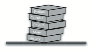
தினசரி வாழ்வில் நிரைய தரவமைப்புகளைக் காணலாம். உதாரணமாக ஒரு மேசை மீது அடுக்கப்பட்ட தட்டுகளை எடுத்துக்கொண்டால், மேலுள்ள தட்டுக்களை எடுத்த பின்னரே கடைசியில் உள்ள கீழ் தட்டை எடுக்கலாம்; ஒரு புத்தகம் அடுக்கபட்டிருக்கையில் மேல் உள்ள நூலின் அட்டைப்படம் மட்டுமே நமக்கு தெரிகிறது; அடுக்கின் கீழுள்ள மற்ற நூல்களை எடுக்க முதல்/மேல் நுலை நாம் எடுக்க நிர்பந்தமாகிறது. இவை இரண்டுமே இயல்புவாழ்கையில் நாம் காணும் சிறிய அடுக்கின் பயன்பாடுகளாகும்.
A stack of books
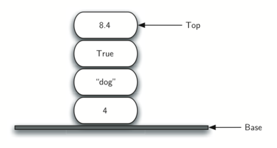
இந்த கீழ்காணும் படத்தில் உள்ள அடுக்கில் பல அடிப்படை பைத்தான் மொழி அடிப்படை தரவுகள் இடல்பெருகிறது:
A stack of primitive Python objects
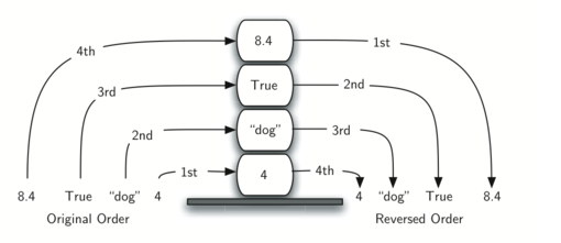
அடுக்கின் முக்கியமான புரிதல்களில் ஒன்றானது, அடுக்கில் நுழைக்கப்படும் உருப்படிகள் அவற்றை அடுக்கிலிருந்து நீக்கும் பொழுது முன்னுக்கு-பின் வரிசை மாரிவருகிறது.
உதாரணமாக ஒரு காலியான மேசையின் மீது ஒரு நூல் அடுக்கை உருவாக்கினால் நீங்கள் முதல் அடுக்கிய நூல் அடுக்கின் கீழ் முடிவு வாயிலில் இருக்கும்: மேலும் அடுக்கில் சில நூல்களை சேர்த்தபின் நூல்களை அடுக்கிலிருந்து எடுத்தால் அவை முன்னுக்குப்பின் வரிசை மாரியிருப்பதைக் காணலாம். இப்படி வரிசை மாற்றத்தை செயல்படுத்தும் சக்தி உள்ளதால் அடுக்குகள் கணிமையில் சிறப்பிடம் பெருகின்றன.
கீழே, அடுக்கின் நிலைமாற்றங்களையும் அதன் உருப்படிகளை அடுக்கில் சேர்க்கும் பொழுதும், நீக்கும் பொழுதும் காணலாம். உருப்படிகளின் வரிசையை கவணிக்கவும்.
கீழே, அடுக்கின் நிலைமாற்றங்களையும் அதன் உருப்படிகளை அடுக்கில் சேர்க்கும் பொழுதும், நீக்கும் பொழுதும் காணலாம். உருப்படிகளின் வரிசையை கவணிக்கவும்.
The reversal property of stacks
அடுக்கின் வரிசைமாற்றமாக்கும் தன்மையைக் இயல்பு வாழ்க்கையில் கணினியை செயல்படுத்தும் சமயம் எங்கு காணலாம் என்று சற்று சிந்த்தித்து பாருங்கள். உதாரணமாக ஒவ்வொரு வலை உலாவியில் "பின் செல்" (back) என்ற ஒரு பொத்தான் இருக்கும். வலை உலாவியின் வழியாக ஒவ்வொரு வலைதளமாக நீங்கள் பயன்படுத்தி செல்லும் பொழுது அந்த்த வலைதளத்தின் முகவரி (உரிலி URL) ஒரு அடுக்கினில் சேர்க்கப்படுகிறது. தற்சமயம் நீங்கள் பயன்படுத்தும் வலைத்தளம் முகவரி அடுக்கின் உச்சியில் உள்ளது; முதல் தொடங்கிய வலைத்தளம் அடுக்கின் கீழ் நிலையில் உள்ளது. "பின் செல்" பொத்தானை அழுத்தும் பொழுது ஒவ்வொரு முறையும் அடுக்கின் எதிர்வரிசையில் உள்ள "பழைய" வலைதளத்திற்கு செல்லும்.
உருவற்ற தகவல் தரவமைப்பு - Stack Abstract Data Type
உருவற்ற தகவல் தரவு வகை (abstract data type, அல்லது ADT), என்பது ஒரு ஏரண அளவில் எப்படி தரவின் அமைப்பை காணலாம், அதில் எண்ணென் சார்புகள் உள்ளன என்றெல்லாம் சொல்லும்; இது தரவமைப்பை பற்றி எதுவும் கூறாது. அதாவது, இந்த நிலையில் எதனை நிலைப்படுத்துகிறோம் என்று மட்டுமே சிந்திக்கிறோம் தவிர எப்படி இதனை கட்டுமானப்படுத்துகிறோம் என்றல்ல. அதாவது "உருவற்ற தகவல் தரவு" (ADT) தகவல்களை தரவுபடுத்துவதை (encapsulation) முன்னிலையாக கொண்டு அதன் நிலைப்படுத்துவதை பொருட்படுத்தாமல் சார்பு செயல்பாடுகளை பற்றி மட்டும் பேசுகிறது.
மாறாக, ஒரு தகவல் தரவமைப்பு (data structure) என்பது ஒரு உருவற்ற தகவல் தரவின் உருவாக்கமாகும்; இதனால் தகவல்களின் ஒரு செயல்படும் சார்பாக ஆக்குகிறது; தகவல் தரவமைப்பு என்பது ஒரு சில/பல எளிமையான தகவல் தரவமைப்பின் வழியாகவும் நிரல் கொட்பாடுகளினாலும் உருவாக்கப்படுகிறது.
கணிமை கேள்விகளை "உருவற்ற தகவல் தரவு" என்ற கோணத்திலும் "தகவல் தரவமைப்பு" என்ற கோணத்திலும் இருவழியாக பார்வையில் காண்பது சிக்கலான கேள்விகளுக்கு ஒரு சிறப்பான விடைகாண, அதிகபடி தகவல் பகிறாமல், வழிவகுகிறது; ஆகையால் ஒரே உருவற்ற தகவல் தரவினை பலவழிகளில் தகவல் தரவமைப்பாக உருவாக்கலாம். இந்த பிரிவினை வழியாக ஒருவரி சிக்கலின் "உருவற்ற தகவல் தரவு" பயன்பாட்டை மாற்றாமல் மற்றொருவர் "தகவல் தரவமைப்பினை" செயல்படுத்தலாம் / அல்லது செயல்பட்டினை மாற்றலாம்.
அடுக்கு என்ற "உருவற்ற தகவல் தரவு" மேலிருந்து உருப்படிகளை சேர்ப்பதும், நீக்குவதும் இதன் முன்னிலை சார்பாகும். அடுக்கு என்பதன் இடைமுகம் கீழ்கண்டவாரு அமைந்திருக்கும்:
- Stack() என்ற கட்டளை ஒரு புதிய அடுக்கினை உருவாக்கும்
- push(பொருள்) பொருள் என்ற ஒரு உருப்படியை அடுக்கின் உச்சியில் சேர்க்கிறது
- pop() அடுக்கின் உச்சியில் உள்ள உருப்படியை நீக்கம் செய்தும் அந்த பொருளை பின்கொடுக்கும்
- peek() அடுக்கின் உச்சியில் உள்ள பொருளை, நீக்கம் செய்யாமல், பின்கொடுக்கும்; அடுக்கு மாற்றப்படாது
- is_empty() அடுக்கினில் ஏதேனும் உருப்படிகள் உள்ளனவா என்றதை பூலியன் வகையாக (மெய்/பொய்) என மெய்ப்பித்து காட்டும்
- size() அடுக்கின் அளவை முழு எண்ணாக காட்டும்
உதாரணம், s என்பது ஒரு புதிதாக உருவாக்கப்பட்ட அடுக்கு என்றால், அதில் உருப்படிகள் ஏதேனும் இல்லை என்றபடியும் அமைந்துள்ளது; அன்னிலையில் அந்த அடுக்கின் மேல் அமைந்த செயல்பாடுகளும் அடுக்கின் நிலை மாற்றங்களையும் கீழ் உள்ள பட்டியல் விளக்குகிறது. அடுக்கின் உச்சி உருப்படியை "அடுக்கு [உள்ளடக்கம்]" என்ற பட்டியலின் வலது புரமாக அமைந்திருக்கும்:
Stack operation | Stack contents | Return value |
s.is_empty() | [] | True |
s.push(4) | [4] | |
s.push('dog') | [4, 'dog'] | |
s.peek() | [4, 'dog'] | 'dog' |
s.push(True) | [4, 'dog', True] | |
s.size() | [4, 'dog', True] | 3 |
s.is_empty() | [4, 'dog', True] | False |
s.push(8.4) | [4, 'dog', True, 8.4] | |
s.pop() | [4, 'dog', True] | 8.4 |
s.pop() | [4, 'dog'] | True |
s.size() | [4, 'dog'] |
இதன் வழி நீங்கள் அடுக்கு மற்றும் அதன் சார்பு செயல்பாட்டினை உணரலாம்.
2.2 அடுக்குகளின் செயற்பாடு - A Stack Implementation
இந்த பகுதியில் ஒரு அடுக்கு தரவமைப்பை பைத்தான் மொழியில் நிரல்படுத்தி பார்க்கலாம். இதுவரை அடுக்கு என்பதில் 'வடிவில்லா தரவமைப்பு வகை' என்பதை மட்டுமே கையாண்டுள்ளோம் - அந்த வகை தரவமைப்பில் இருந்து ஒரு நிரலாக பைத்தானில் செயல்படுத்தினால் அதற்கு 'அடுக்கு தகவல்தரவமைப்பு' என்று நேரடியாக சொல்லலாம்.
பைத்தானில், list, என்ற தகவல் தரவமைப்பின் இயக்கத்தை கொண்டு ஒரு அடுக்கு அமைக்க முடியுமா என்று நீங்கள் என்னலாம். ஆம் - இதனை சரிவர சொல்லவேண்டுமானால், list ”என்பதை அடுக்காகவும் பயன்படுத்தலாம்”. அதாவது, list என்பதன் அம்ச செய்லபாடான .append() என்ற நிரல்பாகத்தை கொண்டு அடுக்கின் உச்சியில் உருப்படிகளை நுழைக்கலாம்.
நடைமுறையில் “பைத்தான் பட்டியலை அடுக்காக பயன்படுத்துவது” என்றபடி அடுக்கினை செயல்படுத்தலாம்; அதாவது, : தோசை_அடுக்கு = [] என்றும் append (பின் இணைக்க) மற்றும் pop (கடைசி நீக்கு) மற்றும் len(தோசை_அடுக்கு) என்று அடுக்கின் நீளம் கணக்கிடவும், மற்றும் தோசை_அடுக்கு[-1] என்று உச்சி உருப்படியை காண (peek) பட்டியலின் செய்ல்பாடுகளை அடுக்காக பயன்படுத்தலாம். பைத்தான் list (பட்டியல்) அடுக்கு என்பதன் அம்சங்களைத்தாண்டி கூடுதல் செயல்பாடுகளை தருகிறது; உதாரணமாக இடம் சூட்டு எண் கொண்டு (index) உருப்படியை அனுகுவது, அல்லது உருப்படியை நுழைக்கவோ நீக்கவோ இயலும்.
நாம் பைத்தான் பட்டியலை அடுக்காக பயன்படுத்தினாலும் அது ஒரு அடுக்கின் வடிவம் மட்டுமே என்று தெளிவாக தெறிவிக்கவேண்டும். சில நேரங்களில் இதை அடுக்கு என்ற மாரியின் பெயர் சூட்டி தெரியப்படுத்திடலாம். மற்ற நேரங்களில் ̀class` வகை ஒன்றினைக் கொண்டு அதற்கு அடுக்கு என பெயரிட்டும் செயல்படலாம் எனில் அதன் உள்செயல்பாடுகள் பட்டியலைக்கொண்டு இயக்கப்பட்டாலும் அதன் புற அம்சங்கள் அடுக்காக தென்படும்.
இவ்வகையான 'abstraction' (உருவிலி வடிவமைப்பு) என்பதே உருவில்லாத தகவல் தரவமைப்பிற்கும் செயல்படுத்தப்பட்ட தகவல் தரவமைப்பிற்கும் உள்ள வித்தியாசம்; கீழே இருவகையாக ஒரு பட்டியலை அடிப்படையாக கொண்டு அடுக்கினை உதாரணம் காட்டுகிறோம்:
மேல் உள்ள உதாரணத்தில் பட்டியலின் வலது வாயிலில் (கடைசியில்) அடுக்கின் உச்சியாகவும் ̀appendஎன்பதைக்கொண்டுpush (உச்சியில் நுழை) என்றும், ̀pop என்பதைக் கொண்டு (உச்சியில் நீக்கு) என்ற அடுக்கின் அம்சங்களை செயல்படுத்தியிருக்கின்றோம்.
கீழ் உள்ள உதாரணத்தில், மாறாக, ̀pop̀, ̀push` உச்சியில் நீக்கு/நுழை என்பதை பட்டியலின் வலது வாயிலில் (முதலில், இடம் 0) இருந்து செயல்படுத்தலாம். :
மேல்கண்டு இருவகையான செயல்பாடுகள் இருந்தாலும் ஒரு பொருளாக அடுக்கின் இடைமுகம் மட்டுமே அளிக்கிறது; இதை 'abstraction' (உருவிலி வடிவமைப்பு) என்பதன் செயல்படுத்தலாக உணரலாம். இரண்டும் ஒரே இடைமுகம் அளித்தாலும் நடைமுறையில் ஒன்றைவிட மற்றொன்று சிக்கனமாக இருக்கிறது. பைத்தான் பட்டியல் செயல்பாடுகள் append மற்றும் pop() இரண்டும் கணிமை சிக்கல் அளவு O(1) என்றாகும். எனவே முதல்படியாக நாம் கடைசி (வலது வாயில்) பட்டியல்வழி கட்டமைத்த அடுக்கினில் எத்தனை உருப்படிகள் இருந்தாலும் அது ஒரே நேரத்தில் நுழைக்கவும், நீக்கவும் செய்யலாம். மாறாக நாம் முதல் (இடது வாயில்) பட்டியல்வழி கட்டமைத்த அடுக்கினில் நுழை, நீக்கு என்ற இரண்டு செயல்பாடுகளும் கணிமை சிக்கல் அளவு O(n என்ற நேரத்தில் (n என்ற அடுக்கின் அளவில்) இயங்கும். ஆகையால் இரண்டு செயல்படுத்தப்பட்டு அடுக்குகளும் ஒரே நுழை நீக்கு என்ற செயல்பாடுகளை இடைமுகப்படித்தினாலும், அவை தெளிவாக இயக்க நேரம் என்ற அளவில் செயல்படுத்தப்பட்ட தீர்வுகளின்படி வித்தியாசமடைகின்றன.
அடுத்த கட்டங்களில் இந்த நூலில் ̀list` என்ற பைத்தான் தரவமைப்பை அடுக்காக நேர்வழியோ செயல்படுத்துவோம் - அடுக்கின் அம்சங்களை மட்டுமே பட்டியலில் செயல்படுத்த கவனம் கொள்ள எச்சரிக்கை எடுத்துக்கொள்ள வேண்டும்:
class Stack: def __init__(self): self._items = [] def is_empty(self): return not bool(self._items) def push(self, item): self._items.append(item) def pop(self): return self._items.pop() def peek(self): return self._items[-1] def size(self): return len(self._items) |
It’s important to note that we could’ve chosen to implement the stack using a list where the top is at the beginning instead of at the end. In this case, instead of using pop and append as above, instead we’d pop from and insert into position 0 in the list. Here’s a possible implementation of that approach:
class Stack: def __init__(self): self._items = [] def is_empty(self): return not bool(self._items) def push(self, item): self._items.insert(0, item) def pop(self): return self._items.pop(0) def peek(self): return self._items[0] def size(self): return len(self._items) |
This ability to change the physical implementation of an abstract data type while maintaining the logical characteristics is an example of abstraction at work. However, even though the stack will work either way, if we consider the performance of the two implementations, there’s definitely a difference. Recall that the append and pop() operations were both O(1) . This means that the first implementation will perform push and pop in constant time no matter how many items are on the stack. The performance of the second implementation suffers in that the insert(0) and pop(0) operations will both require O(n) for a stack of size n. Clearly, even though the implementations are logically equivalent, they would have very different timings when performing benchmark testing.
Going forward, we’ll simply use Python lists directly as stacks, being careful to only use the stack-like behavior of the list.
2.3 சமமான அடைப்புக்குறிகள் - Balanced Parentheses
தற்போது அடுக்குகளைக்கொண்டு கணினி அறிவியலில் உள்ள ஒரு சிக்கலை தீர்வுகாணலாம். கண்டிப்பாக கணித பாடத்தில் இது போன்ற ஒரு கணக்கை எழுதியிருக்கலாம்;
(5+6)×(7+8)/(4+3) (5+6) x (7+8)/(4+3) (5+6)×(7+8)/(4+3)
இங்கு அடைப்புக்குறிகள் ஒரு என்பது எந்த கணித செயல்பாடுகள் இணைந்து செயல்படவேண்டும், எந்த வரிசையில் செயல்படவேண்டும் என்பதை குறிக்கின்றது. மேலும் நீங்கள் லிஸ்பு (Lisp) கணீனி நிரலராக இருந்தால் இப்படியும் சில கணக்கை எழுதியிர்க்கக்கூடும்,
;; இரட்டிப்பு [ எண் ] = எண் * எண்; (defun இரட்டிப்பு(எண்) (* எண் எண்)) |
மேல் உள்ள லிஸ்பு நிரல்பாகம் இரட்டிப்பு என்ற சார்பை குறியீடு செய்கிறது; இந்த சார்பு ஒரு எண்ணை இரட்டிப்பு பெருக்காக - அதாவது தன்னுடன் பெருக்கி விடையளிக்கிறது; இதன் உள்ளீடு ̀எண்̀. லிஸ்பு மொழியில் தாராளமாக அடைப்புக்குறிகள் இருப்பதை காணலாம்.
மேல் உள்ள இரண்டு உதாரணங்களிலும், அடைப்புக்குறிகள் சமமாக வரவேண்டும்; இல்லாவிட்டால் அந்த கணித விதத்திலோ அல்லது அந்த நிரலிலோ ஒரு வடிவ அளவில் ஒரு குறைபாடு/பிழை உள்ளதை குறிக்கும். சமமான அடைப்புக்குறிகள் என்றால் ஒவ்வொரு திறந்த அடைப்புக்குறியிற்கும் இணையான ஒரு மூடு குறியீடு இருக்கும்; மேலும் அடைப்புக்குறிகள் சரியான ஜோடியாக அடுக்கு நிலையில் இருக்கும். உதாரணமாக, கீழ்காண்பவை சமமான அடைப்புக்குறிகள்:
(()()()())
(((())))
(()((())()))
இவற்றை மேலும் கீழுள்ள சர்ங்களுடன் (இவை சமமற்ற சரம்) ஒப்பிட்டு பாருங்கள்:
((((((())
()))
(()()(()
கணினி மொழிகளை பகுப்பாய்வது (parsing) என்ற செயல்முறையிலும் அடைப்புக்குறிகள் சம்மாக உள்ளனவா இல்லையா என்று காண்பது முக்கியமானவை.
சவால் எனில் அடைப்புக்குறிகள் கொண்ட ஒரு சரம் இடதிலுருந்து வலது வரை சமமாக இருக்கிறதா என்பதை கண்டறிவதே. இதனை தீர்வு செய்து ஒரு கணினி நிரல்படுத்த முக்கியமான ஒரு உத்தி இந்த புரிதல் - குறியீடுகளை இடதில் இருந்து வலது வரை அனுகும்பொழுது, சமிபத்திய திறந்த அடைப்புக்குறி அடுத்த மூடும் அடைப்புக்குறியுடன் இணையாக வரவேண்டும். ஆகையால் முதல் அனுகிய திறப்பு அடைப்புக்குறி கடைசி குறியீடு வரை காத்திருக்கவேண்டக்கூடும்.
மூடு அடைப்புக்குறிகள் திறந்த அடைப்புக்குறிகளின் எதிர்வரிசையுல் வடுகிறது; இவை உள்ளிருந்து வெளியே பொருந்துகின்றன. இதுவே கணினி தரவான அடுக்கு தரவமைப்பைக் கொண்டு நிரல்படுத்தலாம் என்ற எண்ணத்தை யூகிக்கிறது.
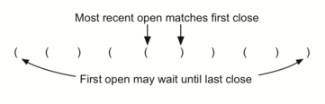
Matching parentheses
அடைப்புக்குறிகள் பொருத்தம் என்பதை அடுக்கு தரவமைப்பு மூலம் நிரல்படுத்திப்பார்க்கலாம்; இந்த செயல்முறையின் சொற்றொடர் எளிதானது. உருப்படிகள் இல்லாத ஒரு அடுக்கினைக் கொண்டு சரங்களை வலம் இருந்து இடது வரை தயார்செய்யுங்கள்; ஒரு குறியீடு திறந்த அடைப்புக்குறி எனில் அதை அடுக்கினுள் நுழைக்கவும் (pop); இதே குறியீட்டின் இணையான மூடு குறியீடு பின்னர காணப்படவேண்டும் என்று குறித்துக்கொள்ளவும். சரத்தில் சந்தித்தகுறியீடு மூடு அடைப்புக்குறியாக இருப்பின் அடுக்கின் நுனியில் உள்ள் உச்சி உருப்படையை நீக்கவும் (pop).
ஒவ்வொரு அடைப்புக்குறியும் திறந்த/மூடப்பட்ட அடைப்புகுறிகளினுள் பொருந்தும் வரை, அடைப்புக்குறிகள் சமமாக இருக்கும். ஒரு முடப்பட்ட அடைப்புக்குறியீடிற்கு இணையான திறந்த அடைப்புக்குறியீடு அடுக்கினுள் இல்லாவிட்டால் அடைப்புக்குறிகள் சமமாக இருக்காது. அடைப்புக்குறிகள் சமமாக உள்ளவரை சரம் முடிவில் அடுக்கில் எந்த உருப்படியும் இருக்காது. இவ்வாரான பைத்தான் நிரல் கீழே காணலாம்:
ஒரு உள்ளிடப்பட்ட சரம் சமமான அடைப்புக்குறிகளை கொண்டதா என்பதை கணிக்க, is_balanced என்ற நிரல் செயல்பாடு மெய் அல்லது பொய் என்ற இரும நிலை ஏரணவகை விடை அளிக்கிறது. தற்சமயம் உள்ளீடு ( எனில் ( திறந்த அடைப்புக்குறி) அது அடுக்கினுள் உச்சியில் நுழைக்கப்படுகிறது; இதை 'push' என்று மற்ற ஆங்கில நூல்களில் காணலாம். தற்சமயம் உள்ளீடு ) எனில் (மூடப்பட்ட அடைப்புக்குறி) அது அடுக்கினுள் உச்சியில் நீக்கப்படுகிறது; இதை 'pop' என்று மற்ற ஆங்கில நூல்களில் காணலாம். ஆனால் அடுக்கினுள் உருப்படிகள் இல்லாத பொழுது இந்த செயல்பாட்டை செய்ய இயலாது; எனினும் நமது உள்ளீட்டினால் இந்நிலையில் வந்தடைந்தோம் - ஆகவே உள்ளீடு சரம் சமமற்ற நிலையில் இருக்கிறது - அதில் திறந்த அடைப்புக்குறிகளைவிட மூடப்பட்ட அடைப்புக்குறிகள் அதிகமாக உள்ளதை நாம் கண்டறியலாம். கடைசியாக, உள்ளீடு சமமாக இருக்கும்வரை அதில் வரக்கூடிய அடைப்புக்குறிகளை நுழைத்தலும் நீக்கலும் சமமாக அமைந்திருக்கும்; இதன் விளைவாக இருதியில் (உள்ளீடு முடிந்தபின்) அடுக்கில் பூச்சியம் உருப்படிகள் காணப்படும். இதுவே சமமான அடைப்புக்குறிகளின் சரம் என்பதன் அறிகுறி.
OPENING = '(' def is_balanced(parentheses): stack = [] for paren in parentheses: if paren == OPENING: stack.append(paren) else: try: stack.pop() except IndexError: # too many closing parens return False return len(stack) == 0 # false if too many opening parens is_balanced('((()))') # => True is_balanced('(()') # => False is_balanced('())') # => False |
சமமான அடைப்புக்குறிகள் பொதுவான தீர்வு - Balanced Symbols: A General Case
The சமமான அடைப்புக்குறிகள் problem shown above is a specific case of a more general situation that arises in many programming languages. The general problem of balancing and nesting different kinds of opening and closing symbols occurs frequently. For example, in Python square brackets, [ and ], are used for lists; curly braces, { and }, are used for dictionaries; and அடைப்புக்குறிகள், ( and ), are used for tuples and arithmetic expressions. It’s possible to mix symbols as long as each maintains its own open and close relationship. Strings of symbols such as
{ { ( [ ] [ ] ) } ( ) }
[ [ { { ( ( ) ) } } ] ]
[ ] [ ] [ ] ( ) { }
are properly சமமான in that not only does each opening symbol have a corresponding closing symbol, but the types of symbols match as well.
Compare those with the following strings that are not சமமான:
( [ ) ]
( ( ( ) ] ) )
[ { ( ) ]
The simple அடைப்புக்குறிகள் checker from the previous section can easily be extended to handle these new types of symbols. Recall that each opening symbol is simply pushed on the stack to wait for the matching closing symbol to appear later in the sequence. When a closing symbol does appear, the only difference is that we must check to be sure that it correctly matches the type of the opening symbol on top of the stack. If the two symbols don’t match, the string isn’t சமமான. Once again, if the entire string is processed and nothing is left on the stack, the string is correctly சமமான.
The Python program to implement this is shown below. The only change is that we use a dictionary to ensure that symbols popped from the stack correctly match our expectations of pairing with the symbol being considered at the time.
PAIRINGS = { '(': ')', '{': '}', '[': ']' } def is_balanced(symbols): stack = [] for s in symbols: if s in PAIRINGS: stack.append(s) continue try: expected_opening_symbol = stack.pop() except IndexError: # too many closing symbols return False if s != PAIRINGS[expected_opening_symbol]: # mismatch return False return len(stack) == 0 # false if too many opening symbols is_balanced('{{([][])}()}') # => True is_balanced('{[])') # => False is_balanced('((()))') # => True is_balanced('(()') # => False is_balanced('())') # => False |
These two examples show that stacks are very important data structures for the processing of language constructs in computer science. Almost any notation you can think of has some type of nested symbol that must be matched in a balanced order. There are a number of other important uses for stacks in computer science. We’ll continue to explore them in the next sections.
2.4 எண்களை நிலைமாற்றல் - Converting Number Bases
கணினி அறிவியில் கற்றலில் இரும (binary) நிலையில் எண்களின் வடிவத்தை பற்றி கற்றிருப்பீர்கள். இரும நிலை குறியீடு என்பது கணினி அறிவியலில் ஒரு முக்கியமான ஒரு கோட்பாடு - எனில் கணினியின் நினைவகத்தில் இரும இலக்குகளான 0 அல்லது 1 என்ற சரங்களாக குறியிடப்பட்டிருக்கும். ஆகையால் தசம எண்களை இயல்பாக பயன்படுத்தும் மனிதர்கள் நாம் கணினியுடன் இரும எண்குறியீட்டில் உரையாட சற்று சிக்கலுக்குள்ளாகியிருப்போம் - எனவே தசம நிலையில் இருந்து ஒரு எண்ணை இரும நிலைக்கும், இரும நிலையில் இருந்து தசம நிலைக்கும் மாற்றம் செய்ய பழகிக்கொண்டோம்; இந்த செயல்முறை எப்படி இயங்குகிறது? அடுக்குகளின் வாயிலாக - பார்க்கலாம் வாங்க.
முழு எண்கள் (Integer) என்றவற்றை அதிகளவில் கணிதபாடத்திலும் கணினிவழியிலும் பயன்படுத்துகிறோம்; இவற்றை பெரும்பாலும் பத்தின் அடிப்படையிலான தசம் குறியீட்டில் கொண்டு செயல்படுகிறோம். உதாரணம் முழு எண். உதாரணம் முழு எண் 23310 என்றும் அதன் இரும குறியீட்டில் (binary equivalent) 111010012111010012 எழுதுகையில் அதன் மதிப்பு ஒரோபடியாக உள்ளது; இதனை கீழ்கண்டவாரு புரிந்துகொள்ளலாம்
2×10²+3×101+3×1002 and 1×27+1×26+1×25+0×24+1×23+0×22+0×21+1×20
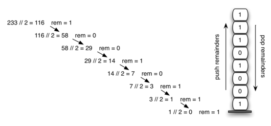
எல்லாம் சரிதான் - ஆனால் இதை நாம் எப்படி ஒரு கணினி செயல்முறையை தானியங்கியாக உருவாகுவது? செய்யலாம்; இதற்கு இரண்டால் வகுத்தல் செயல்முறௌ என்பதை ஒரு அடுக்கின் ஊடாக மிஞ்சும் இலக்குகளை சேமித்தால் இந்த செயல்முறையின் முடிவில் அடுக்கில் நிற்கும் இலக்குகள் அந்த எண்ணின் இரும வெளிப்பாடாகும்.
இரண்டால் வகுத்தல் செயல்முறையில் பூச்சியத்தை விட அதிகமான ஒரு எண்ணில் இருந்து தொடங்குகிறோம் என்ற கட்டுப்பாடு உள்ளது; அடுத்தபடியாக ஒவ்வொரு சுற்றிலும் மீதம் உள்ள எண்ணை இரண்டால் வகுத்தல் செய்து எஞ்சிய மீதம் எண்ணை கையில் கொள்ளலாம். முதன் முதல் இரண்டால் வகுத்தல் மீதம் 1 ஆக இருந்தால் அது ஒற்றைப்படை எண்; அல்லது 0 ஆக இருந்தால் அது இரட்டைப்படை எண். மேலும் அடுத்த படி உள்ள . நமது இரும எண் குறியீட்டை ஒரு இரும இலக்க சரம் ஒன்றில் தொடர் கோர்வையாக உருவாக்கலாம்; முதல் வகுத்தல் மீதம் (remainder) இரும எண் குறியீட்டின் கடைசி இடத்தில் இடம் பெருகிறது. கீழ் கண்டபடி, இந்த வரிசைமாற்றம் என்ற அம்சம் இந்த சிக்கலின் தீர்வில் இடம் பெருவதால் இதனை நிரலாக்கம் செய்வதற்கு அடுக்குகள் உதவும்.
Decimal-to-binary conversion
பைத்தான் நிரல் இரண்டால் வகுத்தல் நிரல்படுத்துகிறது. இதில் convert_to_binary என்ற சார்பு (நிரல்பாகம் அல்லது செயல்பாடு) ஒரு எண் ஒன்றை சார்பின் உள்ளீடாக பெருகிறது; அதன்பின் பலமுறை அது இரண்டால் வகுத்துவருகிறது. வரி 7-இல் பைத்தான் மொழியில் உள்ள (modulo operator) வகுத்தல்மீதம் செயற்குறியை, %, பயன்படுத்தி மீதம் எண்ணை எடுத்து, வரி 8-இல் அதனை அடுக்கினுள் உச்சியில் நுழைக்கிறது. இது பலமுறை நடந்தபின் வகுத்தல் எண் 0 ஆக மாறுகிறது; இச்சமயம் இரும எண் சரம், வரிகள் 11-13, முழுதாக உருவாக்கப்படுகிறது. வரிகள் 11-இல் ஒரு புதுசரம் ஒன்றில் தொடங்குகிறது. இரும இலாக்காக்கள் அடுக்கிலிருந்து நீக்கப்பட்டு சரம் வலது கடைசியில் இணைக்கப்படுகிறது. இந்த சரம் நிரல்பாகம் முடிவின்கன் பின்கொடுக்கப்படுகிறது.
def convert_to_binary(decimal_number): remainder_stack = [] while decimal_number > 0: remainder = decimal_number % 2 remainder_stack.append(remainder) decimal_number = decimal_number // 2 binary_digits = [] while remainder_stack: # we could just reverse and join `remainder_stack` of course, # as it is simply a Python list, but popping off into another # list helps demonstrate that the only behavior we need from # `remainder_stack` is stack-like binary_digits.append(str(remainder_stack.pop())) return ''.join(binary_digits) convert_to_binary(42) # => '101010' |
இதே செயல்முறையை எவ்வித அடிப்படை எண்பதற்கும் அடிப்படை மாற்றம் செய்ய பயன்படுத்தலாம். கணினி அறிவியலில் பலவித அடிப்படை எண்களை பயன்படுத்துகிறோம் - இரும எண் (binary), பதிணாறின் அடிப்படை (hexadeicmal), எட்டின் அடிப்படை (octal) எண் என பலதரப்பட்ட எண்வகைகள் உண்டு.
உதாரணமாக பத்தின் அடிப்படை (பொதுவக தினசரிவாழ்வில் பயன்படுத்தப்படுவது) இதில் எழுதப்பட்ட 233 எண், மற்றும் அதன் எட்டின் அடிப்படை, பதிணாறின் அடிப்படை எண் வடிவங்கள் 3518 மற்றும் E916 என்று எழுதப்படுகின்றன; இதன் பொருளாவது,
3×82 + 5×81 + 1×80 மற்றும் 14×161 + 9×160
DIGITS = '0123456789abcdef' def convert_to_base(decimal_number, base): remainder_stack = [] while decimal_number > 0: remainder = decimal_number % base remainder_stack.append(remainder) decimal_number = decimal_number // base new_digits = [] while remainder_stack: new_digits.append(DIGITS[remainder_stack.pop()]) return ''.join(new_digits) convert_to_base(25, 2) # => '11001' convert_to_base(25, 16) # => '19' |
கணினி நிரல்பாகம், சார்பு, convert_to_binary என்பதை சற்றோ மாற்றினால் அது பத்தின் அடிப்படை மதிப்பை மற்றும் எடுத்துக்கொள்ளாமல் அடிப்படை விதத்தை ஒரு இரண்டாவது உள்ளீடாக எடுத்துக் கொள்ளும். ஏற்கணவே நாம் "இரண்டால் வகுத்தல்" என்ற உத்தியை பொதுப்பாடாக செயல்படுவதற்கு “அடிப்படை-எண் வழியாக வகுத்தல்” என்ற நிலைபாட்டிற்கு மாற்றி செயல்படவேண்டும். இதனை ஒரு புது செயல்பாடாக convert_to_base, கீழ்கண்டபடி உருவாக்கலாம்; இதில் இரண்டாம் உள்ளீடாக அடிப்படை எண் இரண்டில் இருந்து பதிணாறு வரை உள்ள ஒரு மதிப்பை எடுத்துக்கொள்ளும்.
வகுத்தல் அடிப்படை மட்டும் உள்ளீட்டின் மதிப்பாக (ஏற்கணவே இரண்டு என்ற மாறிலி) மற்றப்படுகிறது; மற்றபடி பழையபடி செய்த வகுத்தல் மீதம் அடுக்கினுள் நுழைக்கப்படுவது; பழையபடி செய்தபடி இடதில் இருந்து வலது வரை உள்ளீட்டு சரம் சேர்க்கப்படுகிறது. அடிப்படை எண் 2இல் இருந்து 10வரை உள்ள எண்களுக்கு 0-இல் இருந்து 9-வரை உள்ள எண் இலக்குகள் எளிதாக பயன்படுத்தலாம்; இவை பொதுவான 0, 1, 2, 3, 4, 5, 6, 7, 8, மற்றும் 9 என்ற இலக்குகள். 10-ஐ தாண்டியபின் அடிப்படை எண் என்பதை எப்படி குறியிடுவது? இப்பொழுது வகுத்தல் மீதங்களை 10-இன் அடிப்படையில் பார்த்தால் மீதம் என்பதோ இரண்டு இலக்க எண்ணாக வருகிறது - இது வேலைக்காகாது. மாறாக நாம் வேறு இலக்க எண்களை கொண்டு ஒரு இலக்க குறியீடுக்கு இணங்க செயல்படவேண்டும்.
இந்த சிக்கலுக்கு தீர்வாக என்ன சொல்லலாம் என்றால் இலக்குகளுடன் அகரவரிசை (ஆங்கில) எழுத்துக்களையும் சேர்ப்பது. உதாரணமாக, பதிணாறின் அடிப்படை (hexadecimal) எண்கள் பத்தின் அடிப்படை எண்களையும் முதல் ஆறு ஆங்கில எழுத்துக்களையும் இணைத்து 16 இலக்குகளைக் கொண்டு செயலபடுகிறது. இதனை அடிப்படை மாற்றம் செய்ய, ஒரு இலக்கு சரம் ஒன்றை இந்த பதிணாறின் படி உருவாக்குகிறோம்; அதாவது 0 என்ற இலக்கு 0 இடத்திலும், 1 முதல் இடத்திலும், ... , 9 என்பது ஒன்பதாம் இடத்திலும், A என்பது பத்தாம் இடத்திலும், B என்பது பதினோறாம் இடத்திலும், என்றபடி F என்பது பதினைந்தாம் இடத்திலும் இருக்கும். உதாரணமாக வகுத்தல் மீதம் (remainder) அடுக்கில் இருந்து நீக்கப்பட்ட பின், அதனை இடம் சூட்டு எண்ணாக இலக்கு சரத்தில் அதன் கடைசியில் சேர்க்கலாம். உதாரணமாக,13 என்ற எண் அடுக்கில் இருந்து நீக்கப்பட்டால், அதற்கு இணையான இலக்கம் D சரத்தில் இணைக்கப்படும்.
2.5 Infix, Prefix and Postfix Expressions - நடுஒட்டு, முன்/பின் ஒட்டு சூத்திரங்கள்
When you write an arithmetic expression such as B * C, the form of the expression provides you with information so that you can interpret it correctly. In this case we know that the variable B is being multiplied by the variable C since the multiplication operator * appears between them in the expression. This type of notation is referred to as infix since the operator is in between the two operands that it’s working on.
Consider another infix example, A + B * C. The operators + and * still appear between the operands, but there’s a problem. Which operands do they work on? Does the + work on A and B or does the * take B and C? The expression seems ambiguous.
In fact, you’ve been reading and writing these types of expressions for a long time and they don’t cause you any problem. The reason for this is that you know something about the operators + and *. Each operator has a precedence level. Operators of higher precedence are used before operators of lower precedence. The only thing that can change that order is the presence of parentheses. The precedence order for arithmetic operators places multiplication and division above addition and subtraction. If two operators of equal precedence appear, then a left-to-right ordering or associativity is used.
Let’s interpret the troublesome expression A + B * C using operator precedence. B and C are multiplied first, and A is then added to that result. (A + B) * C would force the addition of A and B to be done first before the multiplication. In expression A + B + C, by precedence (via associativity), the leftmost + would be done first.
Although all this may be obvious to you, remember that computers need to know exactly what operators to perform and in what order. One way to write an expression that guarantees there will be no confusion with respect to the order of operations is to create what’s called a fully parenthesized expression. This type of expression uses one pair of parentheses for each operator. The parentheses dictate the order of operations; there is no ambiguity. There’s also no need to remember any precedence rules.
The expression A + B * C + D can be rewritten as ((A + (B * C)) + D) to show that the multiplication happens first, followed by the leftmost addition. A + B + C + D can be written as (((A + B) + C) + D) since the addition operations associate from left to right.
There are two other very important expression formats that may not seem obvious to you at first. Consider the infix expression A + B. What would happen if we moved the operator before the two operands? The resulting expression would be + A B. Likewise, we could move the operator to the end. We would get A B +. These look a bit strange.
These changes to the position of the operator with respect to the operands create two new expression formats, prefix and postfix. Prefix expression notation requires that all operators precede the two operands that they work on. Postfix, on the other hand, requires that its operators come after the corresponding operands. A few more examples should help to make this a bit clearer:
Infix expression | Prefix expression | Postfix expression |
A + B | + A B | A B + |
A + B * C | + A * B C | A B C * + |
A + B * C would be written as + A * B C in prefix. The multiplication operator comes immediately before the operands B and C, denoting that * has precedence over +. The addition operator then appears before the A and the result of the multiplication.
In postfix, the expression would be A B C * +. Again, the order of operations is preserved since the * appears immediately after the B and the C, denoting that * has precedence, with + coming after. Although the operators moved and now appear either before or after their respective operands, the order of the operands stayed exactly the same relative to one another.
Now consider the infix expression (A + B) * C. Recall that in this case, infix requires the parentheses to force the performance of the addition before the multiplication. However, when A + B was written in prefix, the addition operator was simply moved before the operands, + A B. The result of this operation becomes the first operand for the multiplication. The multiplication operator is moved in front of the entire expression, giving us * + A B C. Likewise, in postfix A B + forces the addition to happen first. The multiplication can be done to that result and the remaining operand C. The proper postfix expression is then A B + C *.
Consider these three expressions again. Something very important has happened. Where did the parentheses go? Why don’t we need them in prefix and postfix? The answer is that the operators are no longer ambiguous with respect to the operands that they work on. Only infix notation requires the additional symbols. The order of operations within prefix and postfix expressions is completely determined by the position of the operator and nothing else. In many ways, this makes infix the least desirable notation to use.
Infix expression | Prefix expression | Postfix expression |
(A + B) * C | * + A B C | A B + C * |
The table below shows some additional examples of infix expressions and the equivalent prefix and postfix expressions. Be sure that you understand how they’re equivalent in terms of the order of the operations being performed.
Infix expression | Prefix expression | Postfix expression |
A + B * C + D | + + A * B C D | A B C * + D + |
(A + B) * (C + D) | * + A B + C D | A B + C D + * |
A * B + C * D | + * A B * C D | A B * C D * + |
A + B + C + D | + + + A B C D | A B + C + D + |
Conversion of Infix Expressions to Prefix and Postfix - குறிமுறை மாற்றம்
So far, we’ve used ad hoc methods to convert between infix expressions and the equivalent prefix and postfix expression notations. As you might expect, there are algorithmic ways to perform the conversion that allow any expression of any complexity to be correctly transformed.
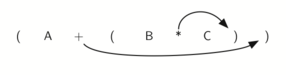
The first technique that we’ll consider uses the notion of a fully parenthesized expression that was discussed earlier. Recall that A + B * C can be written as (A + (B * C)) to show explicitly that the multiplication has precedence over the addition. On closer observation, however, you can see that each parenthesis pair also denotes the beginning and the end of an operand pair with the corresponding operator in the middle.
Look at the right parenthesis in the subexpression (B * C) above. If we were to move the multiplication symbol to that position and remove the matching left parenthesis, giving us B C *, we would in effect have converted the subexpression to postfix notation. If the addition operator were also moved to its corresponding right parenthesis position and the matching left parenthesis were removed, the complete postfix expression would result.
Moving operators to the right for postfix notation
If we do the same thing but instead of moving the symbol to the position of the right parenthesis, we move it to the left, we get prefix notation (below). The position of the parenthesis pair is actually a clue to the final position of the enclosed operator.
Moving operators to the left for prefix notation
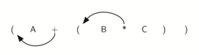
So in order to convert an expression, no matter how complex, to either prefix or postfix notation, fully parenthesize the expression using the order of operations. Then move the enclosed operator to the position of either the left or the right parenthesis depending on whether you want prefix or postfix notation.
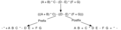
Here’s a more complex expression: (A + B) * C - (D - E) * (F + G):
Converting a complex expression to prefix and postfix notations
General Infix-to-Postfix Conversion - பொதுவான சூத்திரங்கள் குறிமுறை மாற்றம்
We need to develop an algorithm to convert any infix expression to a postfix expression. To do this we’ll look closer at the conversion process.
Consider once again the expression A + B * C. As shown above, A B C * + is the postfix equivalent. We’ve already noted that the operands A, B, and C stay in their relative positions. It is only the operators that change position. Let’s look again at the operators in the infix expression. The first operator that appears from left to right is +. However, in the postfix expression, + is at the end since the next operator, *, has precedence over addition. The order of the operators in the original expression is reversed in the resulting postfix expression.
As we process the expression, the operators have to be saved somewhere since their corresponding right operands are not seen yet. Also, the order of these saved operators may need to be reversed due to their precedence. This is the case with the addition and the multiplication in this example. Since the addition operator comes before the multiplication operator and has lower precedence, it needs to appear after the multiplication operator is used. Because of this reversal of order, it makes sense to consider using a stack to keep the operators until they’re needed.
What about (A + B) * C? Recall that A B + C * is the postfix equivalent. Again, processing this infix expression from left to right, we see + first. In this case, when we see *, + has already been placed in the result expression because it has precedence over * by virtue of the parentheses. We can now start to see how the conversion algorithm will work. When we see a left parenthesis, we’ll save it to denote that another operator of high precedence will be coming. That operator will need to wait until the corresponding right parenthesis appears to denote its position (recall the fully parenthesized technique). When that right parenthesis does appear, the operator can be popped from the stack.
As we scan the infix expression from left to right, we’ll use a stack to keep the operators. This will provide the reversal that we noted in the first example. The top of the stack will always be the most recently saved operator. Whenever we read a new operator, we’ll need to consider how that operator compares in precedence with the operators, if any, already on the stack.
Assume the infix expression is a string of tokens delimited by spaces. The operator tokens are *, /, +, and -, along with the left and right parentheses, ( and ). The operand tokens are the single-character identifiers A, B, C, and so on. The following steps will produce a string of tokens in postfix order.
- Create an empty stack called operation_stack for keeping operators. Create an empty list for output.
- Convert the input infix string to a list by using the string method split.
- Scan the token list from left to right.
- If the token is an operand, append it to the end of the output list.
- If the token is a left parenthesis, push it on the operation_stack.
- If the token is a right parenthesis, pop the operation_stack until the corresponding left parenthesis is removed. Append each operator to the end of the output list.
- If the token is an operator, *, /, +, or -, push it on the operation_stack. However, first remove any operators already on the operation_stack that have higher or equal precedence and append them to the output list.
- When the input expression has been completely processed, check the operation_stack. Any operators still on the stack can be removed and appended to the end of the output list.
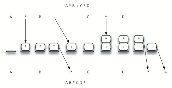
Below we show the conversion algorithm working on the expression A * B + C * D. Note that the first * operator is removed upon seeing the + operator. Also, + stays on the stack when the second * occurs, since multiplication has precedence over addition. At the end of the infix expression the stack is popped twice, removing both operators and placing + as the last operator in the postfix expression.
Converting A * B + C * D to postfix notation
In order to code the algorithm in Python, we’ll use a dictionary called precedence to hold the precedence values for the operators. This dictionary will map each operator to an integer that can be compared against the precedence levels of other operators (we have arbitrarily used the integers 3, 2, and 1). The left parenthesis will receive the lowest value possible. This way any operator that is compared against it will have higher precedence and will be placed on top of it.
PRECEDENCE = { '*': 3, '/': 3, '+': 2, '-': 2, '(': 1 } CHARACTERS = 'ABCDEFGHIJKLMNOPQRSTUVWXYZ' DIGITS = '0123456789' LEFT_PAREN = '(' RIGHT_PAREN = ')' def infix_to_postfix(infix_expression): operation_stack = [] postfix = [] tokens = infix_expression.split() for token in tokens: if token in CHARACTERS or token in DIGITS: postfix.append(token) elif token == LEFT_PAREN: operation_stack.append(token) elif token == RIGHT_PAREN: top_token = operation_stack.pop() while top_token != LEFT_PAREN: postfix.append(top_token) top_token = operation_stack.pop() else: while operation_stack and \ (PRECEDENCE[operation_stack[-1]] >= PRECEDENCE[token]): postfix.append(operation_stack.pop()) operation_stack.append(token) while operation_stack: postfix.append(operation_stack.pop()) return ' '.join(postfix) infix_to_postfix('A * B + C * D') # => 'A B * C D * +' infix_to_postfix('( A + B ) * C - ( D - E ) * ( F + G )') # => 'A B + C * D E - F G + * -' infix_to_postfix('( A + B ) * ( C + D )') # => 'A B + C D + *' infix_to_postfix('( A + B ) * C') # => 'A B + C *' infix_to_postfix('A + B * C') # => 'A B C * +' |
Postfix Evaluation - பின்னொட்டு கணித்தல்
As a final stack example, we’ll consider the evaluation of an expression that’s already in postfix notation. In this case, a stack is again the data structure of choice. However, as you scan the postfix expression, it is the operands that must wait, not the operators as in the conversion algorithm above. Another way to think about the solution is that whenever an operator is seen on the input, the two most recent operands will be used in the evaluation.
To see this in more detail, consider the postfix expression 4 5 6 * +. As you scan the expression from left to right, you first encounter the operands 4 and 5. At this point, you’re still unsure what to do with them until you see the next symbol. Placing each on the stack ensures that they’re available if an operator comes next.
In this case, the next symbol is another operand. So, as before, push it and check the next symbol. Now we see an operator, *. This means that the two most recent operands need to be used in a multiplication operation. By popping the stack twice, we can get the proper operands and then perform the multiplication (in this case getting the result 30).
We can now handle this result by placing it back on the stack so that it can be used as an operand for the later operators in the expression. When the final operator is processed, there will be only one value left on the stack. Pop and return it as the result of the expression. Below we show the stack contents as this entire example expression is being processed.
Stack contents during evaluation
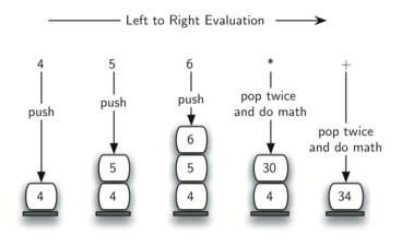
Below we show a slightly more complex example, 7 8 + 3 2 + /. There are two things to note in this example. First, the stack size grows, shrinks, and then grows again as the subexpressions are evaluated. Second, the division operation needs to be handled carefully. Recall that the operands in the postfix expression are in their original order since postfix changes only the placement of operators. When the operands for the division are popped from the stack, they’re reversed. Since division is not a commutative operator, in other words 15/515/515/5 is not the same as 5/155/155/15, we must be sure that the order of the operands is not switched.
A more complex example of evaluation
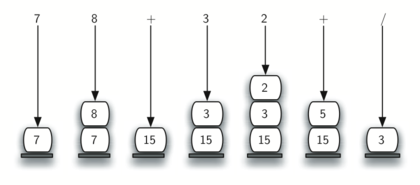
Assume the postfix expression is a string of tokens delimited by spaces. The operators are *, /, +, and - and the operands are assumed to be single-digit integer values. The output will be an integer result.
- Create an empty stack called operand_stack.
- Convert the string to a list by using the string method split.
- Scan the token list from left to right.
- If the token is an operand, convert it from a string to an integer and push the value onto the operand_stack.
- If the token is an operator, *, /, +, or -, it will need two operands. Pop the operand_stack twice. The first pop is the second operand and the second pop is the first operand. Perform the arithmetic operation. Push the result back on the operand_stack.
- When the input expression has been completely processed, the result is on the stack. Pop the operand_stack and return the value.
The complete function for the evaluation of postfix expressions is shown below. To assist with the arithmetic, we importer the handy operator module from the Python standard library to specify functions that will take two arguments and return the result of the proper arithmetic operation.
import operator OPERATION = { '*': operator.mul, '/': operator.div, '-': operator.sub, '+': operator.add } DIGITS = set('0123456789') def evaluate_postfix(postfix_expression): operand_stack = [] for token in postfix_expression.split(): if token in DIGITS: operand_stack.append(int(token)) else: b = operand_stack.pop() a = operand_stack.pop() result = OPERATION[token](a, b) operand_stack.append(result) return operand_stack.pop() evaluate_postfix('7 8 + 3 2 + /') # => 3.0 |
It’s important to note that in both the postfix conversion and the postfix evaluation programs we assumed that there were no errors in the input expression. Using these programs as a starting point, you can easily see how error detection and reporting can be included. We leave this as an exercise.
3. வரிசைத் தரவமைப்பு - Queues
3.1 வரிசைகள் அறிமுகம் - Introduction to Queues
ஒரு வரிசை என்பது உருப்படிகள் வரிசை செய்யப்பட்ட சேகரிப்பு ஆகும்,புதிய உருப்படிகளை சேர்த்தல் ஒரு முனையில் நடைபெறும். அதனை “rear,” என அழைக்கின்றோம்.அதேபோல் உருப்படிகளை நீக்குதல் முனையில் நடைபெறும்.அதனை “front.” என அழைக்கின்றோம்.ஒரு உருப்படியை வரிசையில் நுழைக்கும் போது அது இறுதி முனையில் ஆரம்பித்து முன் முனையை நோக்கிச் செல்லும்.அத்தோடு அடுத்த உருப்படி அகற்றப்படும் நேரம் வரை அது காத்திருக்கின்றது.
வரிசையில் மிகச் சமீபத்தில் சேர்க்கப்பட்ட உருப்படி சேகரிப்பின் இறுதியில் காத்திருக்க வேண்டும். சேகரிப்பில் அதிக நேரம் இருக்கும் உருப்படி முன் முனைக்கு உரியதாகும்.வரிசைப்படுத்தப்படும் கொள்கையானது FIFO, first-in first-out என அழைக்கப்படும். இது “first-come first-served.”("முதலில் வருபவர்களுக்கு முன்னுரிமை") எனவும் அழைக்கப்படலாம்.
ஒரு வரிசையின் எளிய உதாரணம் நாம் அனைவரும் அவ்வப்போது பங்கேற்கும் வழக்கமான வரிசையாகும்.உதாரணமாக திரைப்படத்துக்காக வரிசையில் காத்திருத்தல்,மாளிகைக்கு கடையில் பொருட்களுக்கான பணம்செலுத்தக் காத்திருத்தல்,சிற்றுண்டிச்சாலையில் காத்திருத்தல் போன்றனவாகும்.மிகச் சரியான வரிசைகள் ஒரு புறத்தில் வரிசையா சேரவும் இன்னொரு புறத்தில் வரிசையிலிருந்து வெளியே செல்லவும் கூடியவாறு கட்டுப்படுத்தப்பட்டிருக்கும்.அங்கே வரிசையின் நடுவில் உள்ளே பாய முடியாது. அதேபோல் முன் முனைக்கு வருவதற்கு காத்திருக்காமல் வெளியே போக முடியாது.
A queue of Python data objects
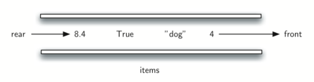
நிஜ வாழ்க்கையில் தரவு ஓட்டத்திற்கு வரிசைகள் மிகவும் பிரபலமான மாதிரிகளாகும்.ஒரு அலுவலகமொன்றில் 30 கணினிகள் மற்றும் அச்சுப்பொறியுடன் கூடிய ஒரு வலையமைப்பைக் கருதுங்கள்.யாராவது அச்சிட விரும்புகிறார்கள் எனின் அவர்களின் அச்சிடும் பணி ஏற்கனவே அச்சிடும் பணிக்காக வரிசையில் சேர்க்கப்படும்.முதலில் உள்ள பணி முதலில் செய்யப்படும். நீங்கள் வரிசையில் கடைசியில் இருந்தால் உங்களுக்கு முன்னுள்ள அனைவரினதும் அச்சிடும் பணி நிறைவடையும் வரை நீங்கள் கட்டாயம் காத்திருக்க வேண்டும்.
கணனி இயக்க அமைப்புகள் ஒரு கணினியில் உள்ள செயல்முறைகளைக் கட்டுப்படுத்த பல்வேறு வரிசைகளைப் பயன்படுத்துகின்றன.அது அடுத்து என்ன செய்ய வேண்டும் என்பதற்கான திட்டமிட,பொதுவாக நிரல்களை இயக்க முயற்சிக்கும் ஒரு வரிசை வழிமுறையை அடிப்படையாகக் கொண்டது முடிந்தவரை விரைவாகவும், முடிந்தவரை பல பயனர்களுக்கு சேவை செய்யவும் மேலும், நாம் தட்டச்சு செய்யும் போது,சில நேரங்களில் விசை அழுத்தங்கள் எழுத்துக்கள் தோன்றுவதற்கு முன்னால் வரும்.கணினி திரை அந்த நேரத்தில் மற்ற வேலைகளைச் செய்வதே இதற்குக் காரணமாகும்.வரிசை போன்ற இடையகத்தில் விசை அழுத்தங்கள் வைக்கப்படுகின்றன இறுதியில் சரியான வரிசையில் திரையில் காட்டப்படும்.
3.2 வரிசை தகவல் தரவமைப்பு - The Queue Abstract Data Type
ஒரு வரிசை, வரிசைப்படுத்தப்பட்ட உருப்படிகள் ஒரு வரிசையில் கட்டமைக்கப்பட்டுள்ளது, அவை ஒரு முனையில் சேர்க்கப்படுகின்றன, அவை “rear,” என்று அழைக்கப்படுகின்றன, மறுமுனையில் இருந்து அகற்றப்படுகின்றன, “front.”. என அழைக்கப்படுகின்றன.வரிசை செயல்பாடுகள்:
- Queue() காலியாக இருக்கும் ஒரு புதிய வரிசையை உருவாக்குகிறது. இதற்கு செயலுருக்கள் தேவையில்லை மற்றும் ஒரு வெற்று வரிசையை பதிலாக வழங்குகிறது.
- enqueue(item) வரிசையின் பின்புறத்தில் ஒரு புதிய உருப்படியைச் சேர்க்கிறது. அதற்கு உருப்படி தேவை மற்றும் எதையும் திருப்பித் தரவில்லை.
- dequeue() வரிசையில் இருந்து முன் உருப்படியை நீக்குகிறது. இதற்கு செயலுருக்கள் தேவையில்லை மற்றும் உருப்படியை பதிலாக வழங்குகிறது. வரிசை மாற்றப்பட்டுள்ளது.
- is_empty() வரிசை காலியாக உள்ளதா என்பதை அறிய பயன்படும்.. இதற்கு செயலுருக்கள் தேவையில்லை மற்றும் பூலியன் பதிலாக வழங்குகிறது.
- size() வரிசையில் உள்ள பொருட்களின் எண்ணிக்கையை வழங்குகிறது. இதற்கு செயலுருக்கள் தேவையில்லை மற்றும் ஒரு முழு எண்ணை பதிலாக வழங்குகிறது.
உதாரணமாக, q என்பது ஒரு வரிசை, மற்றும் அது தற்போது காலியாக உள்ளது என்று நாம் கருதினால், பின்னர் வரிசை செயல்பாடுகளின் வரிசை முடிவுகள். வரிசையின் உள்ளடக்கங்கள் என்பவற்றை கீழே உள்ள அட்டவணை காட்டுகிறது.முன்புறம் வலதுபுறம் இருப்பது போல் காட்டப்பட்டுள்ளது. 4 என்னும் உருப்படியானது ஒருதிசை முனையின் முதல் உருப்படியாக.எனவே இது இருதிசை முனை மூலம் திரும்பிய முதல் உருப்படி.
Queue Operation | Queue Contents | Return Value |
q.is_empty() | [] | True |
q.enqueue(4) | [4] | |
q.enqueue('dog') | ['dog', 4] | |
q.enqueue(True) | [True, 'dog', 4] | |
q.size() | [True, 'dog', 4] | 3 |
q.is_empty() | [True, 'dog', 4] | False |
q.enqueue(8.4) | [8.4, True, 'dog', 4] | |
q.dequeue() | [8.4, True, 'dog'] | 4 |
q.dequeue() | [8.4, True] | 'dog' |
q.size() | [8.4, True] | 2 |
3.3 A Queue Implementation- வரிசை செயற்படுத்தல்
ஒரு அடுக்கியைப் போலவே, "ஒரு பைதான் பட்டியலை ஒரு வரிசையில் பயன்படுத்தவும்" முடியும். மீண்டும், வரிசை சுருக்க தரவு வகையை வரையறுக்கும் குறுகிய நடத்தைகளை விளக்கும் நோக்கத்திற்காக, ஒரு உள் பட்டியலின் விரும்பிய செயல்பாட்டை மட்டுமே வெளிப்படுத்த ஒரு வரிசை வகுப்பை நாங்கள் வரையறுக்கிறோம்.
ஒரு அடுக்கியைப் போலல்லாமல், பைதான் பட்டியலை வரிசையாகப் பயன்படுத்துவதன் செயல்திறன் குறிப்பிடத்தக்கதாகும். கீழே காட்டப்பட்டுள்ள செயலாக்கம் ஒரு புதிய உருப்படியைச் சேர்க்க insert(0, item) பயன்படுத்துகிறது, இது O (n) செயல்பாடாக இருக்கும்.
class Queue(object): def __init__(self): self._items = [] def is_empty(self): return self._items == [] def enqueue(self, item): self._items.insert(0, item) def dequeue(self): return self._items.pop() def size(self): return len(self._items) |
நடைமுறையில், பல பைதான் நிரல் உருவாக்குபவர் நிலையான நூலகத்தின் collections.deque வகுப்பு ஒருதிசை வரிசை மற்றும் இருதிசை வரிசையின் O(1) ஐ அடைய பயன்படுத்துவார்கள். அடுத்த அத்தியாயத்தில் இருதிசை வரிசையை ஆழமாகப் பார்ப்போம்; இப்போது இருதிசை வரிசையைஒரு அடுக்கு மற்றும் ஒரு வரிசையின் கலவையாகக் கருதுகிறது.இது O (1) இரு முனைகளிலிருந்தும் தள்ளும் மற்றும் மேலெழும்புகிறது.
3.4 அவிச்ச கிழங்கு விளையாட்டு ஒத்திகை - Simulating Hot Potato
செயலில் வரிசையைக் காண்பிப்பதற்கான பொதுவான பயன்பாடுகளில் ஒன்று, FIFO முறையில் தரவை நிர்வகிக்க வேண்டிய ஒரு உண்மையான சூழ்நிலையை உருவகப்படுத்துவதாகும்.தொடங்க, குழந்தைகளின் விளையாட்டான அவிச்ச கிழங்கை (Hot Potato) கருத்தில் கொள்வோம். இந்த விளையாட்டில், குழந்தைகள் ஒரு வட்டத்தில் வரிசையில் நிற்கிறார்கள் மற்றும் ஒரு உருப்படியை அண்டை வீட்டிலிருந்து அடுத்தவருக்கு தங்களால் முடிந்தவரை விரைவாக அனுப்புகிறார்கள். விளையாட்டின் ஒரு குறிப்பிட்ட கட்டத்தில், நடவடிக்கை நிறுத்தப்பட்டு உருப்படியை (உருளைக்கிழங்கு) வைத்திருக்கும் குழந்தை வட்டத்திலிருந்து அகற்றப்படும். ஒரே ஒரு குழந்தை எஞ்சியிருக்கும் வரை விளையாட்டு தொடர்கிறது
A six person game of hot potato
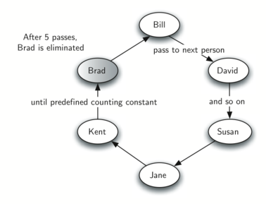
இந்த விளையாட்டு புகழ்பெற்ற Josephus பிரச்சனைக்கு சமமான நவீன தீர்வாகும்.முதல் நூற்றாண்டின் புகழ்பெற்ற வரலாற்றாசிரியர் Flavius Josephus பற்றிய புராணத்தின் அடிப்படையில் Josephus , ரோமுக்கு எதிரான யூத கலகத்தில் கதை சொல்லப்பட்டது,Josephus மற்றும் அவரது 39 தோழர்கள் ரோமானியர்களுக்கு எதிராக ஒரு குகையில் இருந்தனர்.தோல்வி நெருங்குவதால், அவர்கள் மானியர்களுக்கு அடிமைகள் ஆவதைவிட இறப்பது நல்லது என்று முடிவு செய்தனர். அவர்கள் தங்களை ஒரு வட்டத்தில் ஏற்பாடு செய்தனர். ஒரு மனிதன் இருந்தார் நம்பர் ஒன் என்று குறிப்பிடப்பட்டு, கடிகார திசையில் அவர்கள் ஒவ்வொருவரையும் கொன்றனர்ஏழாவது மனிதன். Josephus , புராணத்தின் படி, மற்றவற்றுடன் இருந்தார் அவர் ஒரு திறமையான கணிதவியலாளர். அவர் எங்கு இருக்க வேண்டும் என்பதை உடனடியாக கண்டுபிடித்தார் கடைசியாக போகும் பொருட்டு உட்கார வேண்டும். நேரம் வந்தபோது, தன்னைக் கொள்வதற்குப் பதிலாக அவர் ரோமானியப் பக்கத்தில் சேர்ந்தார். நீங்கள் இந்த கதையின் பதிப்புகள் பலவற்றைக் காணலாம். சிலர் ஒவ்வொரு மூன்றாவது மனிதனையும் எண்ணுகிறார்கள் மற்றும் சிலர் கடைசி மனிதன் குதிரையில் தப்பிக்க அனுமதிக்கிறார்கள் . எந்தவொரு சந்தர்ப்பத்திலும், யோசனை ஒன்றே.ame.
Hot Potato விளையாட்டின் பொதுவான உருவகப்படுத்துதல் ஐ நாங்கள் செயல்படுத்துவோம். எங்கள் திட்டம் பெயர்களின் பட்டியலையும் ஒரு மாறிலியையும் உள்ளிடும், இதை “num,” என்று அழைக்க வேண்டும். இது எண்ணுதலுக்காக பயன்படும். “num,” மூலம் மீண்டும் மீண்டும் எண்ணுவதால்,இது கடைசியாக மீதமுள்ள நபரின் பெயரை வழங்கும்.
வட்டத்தை உருவகப்படுத்த, நாங்கள் ஒரு வரிசையைப் பயன்படுத்துவோம். உருளைக்கிழங்கை வைத்திருக்கும் குழந்தை வரிசையின் முன்னால் இருக்கும் என்று வைத்துக்கொள்ளுங்கள். உருளைக்கிழங்கைக் கடந்து செல்லும் போது, உருவகப்படுத்துதல் வெறுமனே இருதிசை முனைவாக மற்றும் உடனடியாக அந்த குழந்தையை வரிசையின் முடிவில் வைக்கும். மற்ற அனைவரும் முன்னால் இருக்கும் வரை அவள் காத்திருப்பாள், அது மீண்டும் அவளது முறை. எண் செயல்பாட்டிற்குப் பிறகு, முன்புறத்தில் உள்ள குழந்தை நிரந்தரமாக அகற்றப்பட்டு மற்றொரு சுழற்சி தொடங்கும். ஒரே ஒரு குழந்தை இருக்கும் வரை இந்த செயல்முறை தொடரும் (வரிசையின் அளவு 1).
A queue implementation of hot potato
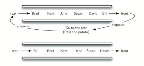
இந்த உருவகப்படுத்துதலின் சாத்தியமான செயல்படுத்தல்:
இந்த எடுத்துக்காட்டில் பட்டியலில் உள்ள பெயர்களின் எண்ணிக்கையை விட எண்ணும் மாறிலியின் மதிப்பு அதிகமாக இருப்பதை கவனிக்கவும்.வரிசை ஒரு வட்டம் போல் செயற்பட்டு மதிப்பை அடையும் வரை ஆரம்பத்திலிருந்து தொடர்ந்து எண்ணும்வரை பிரச்சனை இல்லை .மேலும், பட்டியல் வரிசையில் சேர்க்கப்பட்டுள்ளதைக் கவனிக்கவும். பட்டியலின் முதல் பெயர் வரிசையில் முன்னால் இருக்கும். இந்த சந்தர்ப்பத்தில் Bill பட்டியலின் முதல் உருப்படி ஆக இருப்பதோடு வரிசையின் முன்னால் நகர்கிறது.
இதனை இவ்வாறு நிரல் எழுதலாம்:
from collections import deque def hot_potato(names, num): queue = deque() for name in names: queue.appendleft(name) while len(queue) > 1: for _ in range(num): queue.appendleft(queue.pop()) queue.pop() return queue.pop() hot_potato(('Bill', 'David', 'Susan', 'Jane', 'Kent', 'Brad'), 9) # => 'David' |
இந்த நிரலில் 9 என்ற எண் பட்டியலின் நீளத்தை தாண்டி உள்ளதை கவணத்தில் கொள்ளலாம். இது வரிசை தரவமைப்பில் ஒரு சிக்கல் இல்லை - காரணம் - 9 என்ற வரிசை எண்ணிக்கை வரிசயின் முடிவில் சென்றால் வட்டமாக சுற்றை முடித்த பின் வரிசையின் முதலில் இருந்து எண்ணிக்கை தொடர்கிறது; 6-(9%6)-1. நிரல்படி hot_potato என்ற சார்பு உள்ளீடு பட்டியல் இடதில் இருந்து வலது வரை வரிசையில் முதலில் சேர்க்கப்படுகிறது. இந்த பட்டியலில் 'Bill’ என்ற பெயர் வரிசையின் முதலில் இணைகிறது.
4. இருதிசை வரிசைகள் - Dequeues
"decks" என்று வாசிக்கவேண்டும் - double-ended queue - அதாவது இருதிசை வரிசைகள்
4.1 இருதிசை வரிசை அறிமுகம் - Introduction to Deques
இருதிசை வரிசை(deque),இரட்டை முனை வரிசை என்றும் அழைக்கப்படும், வரிசையைப் போன்ற பொருட்களின் வரிசைப்படுத்தப்பட்ட சேகரிப்பு ஆகும். இது இரண்டு முனைகள், ஒரு முன் மற்றும் பின்புறம், மற்றும் பொருட்கள் சேகரிப்பில் நிலைத்திருக்கும். பொருட்களைச் சேர்ப்பதற்கும் அகற்றுவதற்கும் தடையற்ற தன்மை ஒரு இருதிசை வரிசை(deque)யை வேறுபடுத்துகிறது. புதிய உருப்படிகளை முன் அல்லது பின்புறம் சேர்க்கலாம். அதேபோல, இருக்கும் உருப்படிகளை இரு முனைகளிலிருந்தும் அகற்றலாம். ஒரு வகையில், இந்த கலப்பின நேரியல் அமைப்பு ஒரு தரவு கட்டமைப்பில் அடுக்குகள் மற்றும் வரிசைகளின் அனைத்து திறன்களையும் வழங்குகிறது.
A deque of Python data objects
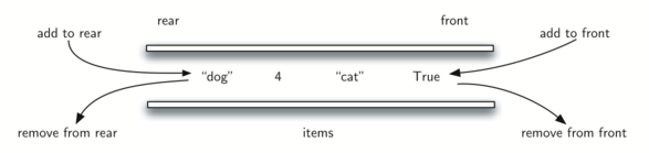
4.1.1 இருதிசை வரிசை தகவல்தரவமைப்பு - The Deque Abstract Data Type
இருதிசை வரிசை சுருக்க தரவு வகை பின்வரும் கட்டமைப்பு மற்றும் செயல்பாடுகளால் வரையறுக்கப்படுகிறது.ஒரு இருதிசை வரிசை ஒழுங்கமைக்கப்பட்டது .மேலே விவரிக்கப்பட்டுள்ளபடி, ஒரு உருப்படிகளின் வரிசைப்படுத்தப்பட்ட தொகுப்பாக, முன் அல்லது பின்புறம் இரு முனைகளிலிருந்தும் உருப்படிகள் சேர்க்கப்பட்டுதலும் அகற்றப்படுதலும் நடைபெறும் . இருதிசை வரிசையின் செயல்பாடுகள் கீழே கொடுக்கப்பட்டுள்ளன.
- Deque() காலியாக இருக்கும் ஒரு புதிய இரு முனைச் சாரையை உருவாக்குகிறது.இதற்கு எந்த செயலுருபும் தேவையில்லை மற்றும் வெற்று இருதிசை வரிசையை பதிலாக(return).தருகின்றது
- add_front(item) இரு முனைச் சாரையின் முன் ஒரு புதிய உருப்படியை சேர்க்கிறது. அதற்கு உருப்படி தேவை மற்றும் எதையும் பதிலாக திருப்பித் தருவதில்லை.
- add_rear(item) இரு முனைச் சாரையின் பின்புறத்தில் ஒரு புதிய உருப்படியை சேர்க்கிறது. அதற்கு உருப்படி தேவை மற்றும் எதையும் பதிலாக திருப்பித் தருவதில்லை.
- remove_front()இரு முனை சாரையிலிருந்து முன்புற உருப்படியை நீக்குகின்றது.இதற்க்கு செயலுரு தேவைப்படாத அதேநேரம் இது நீக்கப்படட உருப்படியை பதிலாக திருப்பித் தரும்.அத்தோடு இரு முனை சாரை மாற்றம் அடைந்திருக்கும்.
- remove_rear() இரு முனை சாரையிலிருந்து பின்புற உருப்படியை நீக்குகின்றது.இதற்க்கு செயலுரு தேவைப்படாத அதேநேரம் இது நீக்கப்படட உருப்படியை பதிலாக திருப்பித் தரும்.அத்தோடு இரு முனை சாரை மாற்றம் அடைந்திருக்கும்.
- is_empty() இரு முனை சாரை காலியாக இருக்கிறதா என்று சோதிக்கிறது. இதற்கு செயலுருக்கள் தேவையில்லை மற்றும் பூலியன் மதிப்பை பதிலாக திருப்பி வழங்குகிறது.
- size() இரு முனை சாரை இல் உள்ள உருப்படிகளின் எண்ணிக்கையை அளிக்கிறது. இதற்கு செயலுருக்கள் தேவையில்லை மற்றும் ஒரு முழு எண்ணை(integer) பதிலாக திருப்பி வழங்குகிறது.
உதாரணமாக, d என்பது உருவாக்கப்பட்ட ஒரு இரு முனை சாரை மற்றும் அது தற்போது காலியாக உள்ளது என்று நாம் கருதினால், கீழேயுள்ள அட்டவணை தொடர்ச்சியான செயல்பாடுகளின் முடிவுகளைக் காட்டுகிறது.
Deque Operation | Deque Contents | Return Value |
d.is_empty() | [] | True |
d.add_rear(4) | [4] | |
d.add_rear('dog') | ['dog', 4] | |
d.add_front('cat') | ['dog', 4, 'cat'] | |
d.add_front(True) | ['dog', 4,'cat', True] | |
d.size() | ['dog', 4, 'cat', True] | 4 |
d.is_empty() | ['dog', 4, 'cat', True] | False |
d.add_rear(8.4) | [8.4, 'dog', 4, 'cat',True] | |
d.remove_rear() | ['dog', 4, 'cat', True] | 8.4 |
d.remove_front() | `['dog', 4, 'cat'] | True |
4.2 இருதிசை வரிசை செயற்படுத்தல் - A Deque Implementation
நடைமுறையில், பைத்தானில் ஒரு இருதிசை வரிசை(deque) ஐப் பயன்படுத்துவதற்கான மிக நேரடியான வழி சேகரிப்பு(collections ) தொகுதியிலிருந்து இருதிசை வரிசை(deque) ஐ இறக்குமதி செய்வதாகும். எவ்வாறாயினும், விளக்க நோக்கங்களுக்காக, கீழே உள்ள ஒரு உருவுள்ள(concrete) தரவு வகையாக பைதான் பட்டியலைப் பயன்படுத்தி ஒரு சாத்தியமான செயல்படுத்தலை நாங்கள் முன்வைக்கிறோம்.
class Deque(object): def __init__(self): self._items = [] def is_empty(self): return self._items == [] def add_front(self, item): self._items.append(item) def add_rear(self, item): self._items.insert(0,item) def remove_front(self): return self._items.pop() def remove_rear(self): return self._items.pop(0) def size(self): return len(self._items) |
remove_front இல் கடைசி உறுப்பை பட்டியலில் இருந்து அகற்றுவதற்குpop முறையைப் பயன்படுத்துகிறோம். இருப்பினும், remove_rear இல்,pop (0)முறை ஆனது பட்டியலில் இருந்து முதல் உறுப்பை கட்டாயம் அகற்ற வேண்டும். அதேபோல், நாம் insert முறையை add_rear இல்` பயன்படுத்த வேண்டும்.இணைக்கும் (apend) முறை பட்டியலின் முடிவில் ஒரு புதிய உறுப்பைச் சேர்ப்பதாகக் கருதப்படுகின்றது.
அடுக்குகள்(stacks ) மற்றும் வரிசைகளை (queues) விபரிப்பிற்கான பைதான் நிரலில் பல ஒற்றுமைகளை நீங்கள் காணலாம். இந்த செயலாக்கத்தில் முன்னால் இருந்து உறுப்புக்களை சேர்ப்பது மற்றும் நீக்குவது O (1) ஆனால் பின்புறத்திலிருந்து சேர்ப்பது மற்றும் நீக்குவது O (n) என்பதை நீங்கள் அவதானிக்கலாம். உறுப்புக்களை சேர்ப்பதற்கும் அகற்றுவதற்கும் தோன்றும் பொதுவான செயல்பாடுகளால் இது எதிர்பார்க்கப்படுகிறது.மீண்டும், முக்கியமான விஷயம் என்னவென்றால், செயல்பாட்டில் முன் மற்றும் பின்புறம் எங்கு ஒதுக்கப்பட்டுள்ளது என்பது எங்களுக்குத் தெரிய வேண்டும்.
4.3 விகடகவி பரிசோதனை - Palindrome Checker
இருதிசை வரிசை தரவு அமைப்பை பயன்படுத்தி எளிதில் தீர்க்கக்கூடிய ஒரு சுவாரஸ்யமான பிரச்சனை உன்னதமான இருவழி ஒக்குஞ்சொல் ( palindrome )பிரச்சனை ஆகும். ஒரு சரத்தினை முன்னோக்கி மற்றும் பின்னோக்கி வாசிக்கும் ஒரே மாதிரியாக இருப்பின் அது இருவழி ஒக்குஞ்சொல் ( palindrome ) ஆகும். எடுத்துக்காட்டாக radar, toot, மற்றும் madam. நாங்கள் குறியிருக்களைக் கொண்ட சரம் ஒன்றினை உள்ளீடாக வழங்கும் போது அது இருவழி ஒக்குஞ்சொல்லா( palindrome ) என்று கண்டறிய ஒரு வழிமுறையை உருவாக்க விரும்புகின்றோம்.
இந்த சிக்கலுக்கான தீர்வு சரத்தின் குறியுருக்களை சேமிக்க ஒரு இருதிசை வரிசையை பயன்படுத்தும்.நாம் சரத்தை இடமிருந்து வலமாகச் செயலாக்கி ஒவ்வொரு குறியுருவையும் இருதிசை வரிசையின் பின்புறமா சேர்க்க வேண்டும்.இந்த கட்டத்தில், இருதிசை வரிசை ஒரு சாதாரண வரிசை போல் செயல்படுகிறது.எனினும்,நாம் இப்போது இருதிசை வரிசையின் இரட்டை செயல்பாட்டை பயன்படுத்த முடியும். இருதிசை வரிசையின் முன்புறம் சரத்தின் முதல் குறியுருவையும் பின்புறம் சரத்தின் கடைசி குறியுருவையும் கொண்டிருக்கும்.
Deque-based is_palindrome strategy
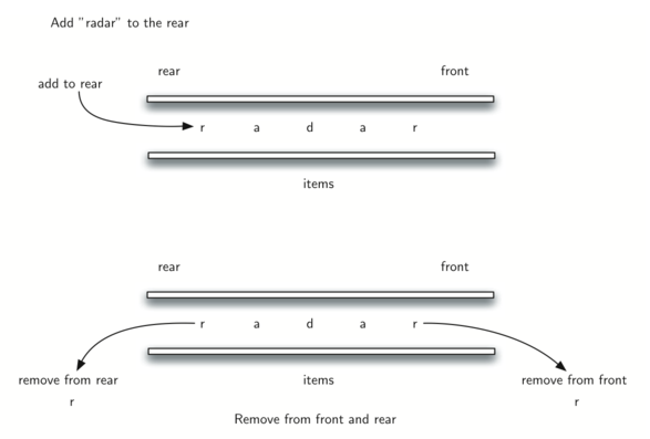
இரண்டையும் நாம் நேரடியாக நீக்க முடியும் என்பதால், அவற்றை ஒப்பிட்டுப் பொருத்தினால் மட்டுமே தொடர முடியும். முதல் மற்றும் கடைசி உருப்படிகளை நாம் பொருத்திப் பார்க்க முடிந்தால், சரத்தின் நீளம் இரட்டைப்படை (even ) அல்லது ஒற்றைப்படை(odd ) இருக்கிறதா என்பதைப் பொறுத்து இறுதியில் குறியுருக்கள் இல்லாமல் போகும்வரை அல்லது இருமுனை சாரையின் அளவு 1 ஆகும்வரை செயற்பாடுடை நிகழ்த்த வேண்டி இருப்போம். எந்தவொரு சந்தர்ப்பத்திலும், சரம் ஒரு இருவழி ஒக்குஞ்சொல்லாக ( palindrome ) இருக்க வேண்டும். இந்த மூலோபாயத்திற்கான முழுமையான செயல்படுத்தல் இதுபோல் தோன்றலாம்:
from collections import deque def is_palindrome(characters): character_deque = deque(characters) while len(character_deque) > 1: first = character_deque.popleft() last = character_deque.pop() if first != last: return False return True is_palindrome('lsdkjfskf') # => False is_palindrome('radar') # => True |
5. பட்டியல் - Lists
5.1 பட்டியல் அறிமுகம் - Introduction to Lists
அடிப்படை தரவு கட்டமைப்புகளின் கலந்துரையாடல் முழுவதும், வழங்கப்பட்ட சுருக்க தரவு வகைகளை செயல்படுத்த பைதான் பட்டியல்களைப் பயன்படுத்தினோம். துரதிருஷ்டவசமாக, "பட்டியல்" இந்த சேகரிப்பு வகைக்கு சிறந்தது அல்ல, விரைவில் நாம் பார்ப்போம் (ஒரு சிறந்த "வரிசை" ஐ ).
பட்டியல் _ சுருக்கம் தரவு வகை_ பற்றி விவாதிக்கும்போது, பட்டியலை ஒரு தொகுப்பாக நாங்கள் கருதுகிறோம் ஒவ்வொரு உருப்படியும் மற்றவற்றுடன் தொடர்புடைய உறவு நிலையை வைத்திருக்கும் உருப்படிகளாகும்.
ஒரு பட்டியலின் உறுப்பினர்கள் பொதுவாக முனைகளாக குறிப்பிடப்படுகிறார்கள்.ஒவ்வொரு முனையிலும் பட்டியலில் உள்ள அடுத்த முனைக்கு ஒரு குறிப்பு இருக்கும்போது, நாங்கள் இதை தனியாக இணைக்கப்பட்ட பட்டியல் என்று அழைக்கிறோம். ஒவ்வொரு முனையிலும் பட்டியலில் அடுத்த மற்றும் முந்தைய முனைகள் இரண்டிற்கும் குறிப்பு இருக்கும்போது, இதை இரட்டிப்பாக இணைக்கப்பட்ட பட்டியல் என்று அழைக்கிறோம்.
எளிமைக்காக, பட்டியல்களில் நகல் உருப்படிகள் இருக்கக்கூடாது என்று கருதுவோம். மீண்டும் இது பைத்தானின் சொந்தப் பட்டியல் வகையிலிருந்து புறப்படும் ஒரு புள்ளியாகும்.
இந்த அத்தியாயத்தில் நாம் வரிசைப்படுத்தப்படாத மற்றும் வரிசைப்படுத்தப்பட்ட பட்டியல்களைக் கருத்தில் கொள்வோம்.நாம் பார்ப்பது போல், ஒரு வரிசைப்படுத்தப்பட்ட பட்டியல் வெறுமனே கூடுதல் செயல்பாடு கொண்ட ஒரு பட்டியல் ஆகும்.அது ஒரு குறிப்பிட்ட வரிசையில் அதன் தொகுதி முனைகளை பராமரிக்க வடிவமைக்கப்பட்டுள்ளது.
5.1.1 சீரிலா பட்டியல் உருவற்ற தரவமைப்பு அம்சங்கள் - The Unordered List Abstract Data Type
மேலே விவரிக்கப்பட்டுள்ளபடி, வரிசைப்படுத்தப்படாத பட்டியலின் அமைப்பு ஒரு தொகுப்பாகும் ஒவ்வொரு உருப்படியும் மற்றைய உருப்படிகளுடன் தொடர்புடைய நிலையை வைத்திருக்கும். சில சாத்தியமான வரிசைப்படுத்தப்படாத பட்டியல் செயல்பாடுகள் கீழே கொடுக்கப்பட்டுள்ளன.
- List() காலியாக இருக்கும் புதிய பட்டியலை உருவாக்குகிறது. இதற்கு செயலுருக்கள் தேவையில்லை மற்றும் ஒரு வெற்று பட்டியலை வழங்குகிறது.
- add(item) பட்டியலில் ஒரு புதிய உருப்படியை சேர்க்கிறது. அதற்கு உருப்படி தேவை மற்றும் எதையும் திருப்பித் தரவில்லை. உருப்படி ஏற்கனவே பட்டியலில் இல்லை என்று வைத்துக்கொள்ளுங்கள்.
- remove(item) பட்டியலிலிருந்து உருப்படியை நீக்குகிறது. அதற்கு உருப்படி தேவை மற்றும் பட்டியலை மாற்றுகிறது. உருப்படி பட்டியலில் உள்ளது என்று வைத்துக்கொள்ளுங்கள்.
- search(item) பட்டியலில் உள்ள உருப்படியைத் தேடுகிறது. அதற்கு உருப்படி தேவை மற்றும் ஒரு பூலியன் மதிப்பை வழங்குகிறது.
- is_empty() பட்டியல் காலியாக உள்ளதா என சோதனை செய்கிறது . அதற்கு செயலுருக்கள் தேவையில்லை மற்றும் பூலியன் மதிப்பை வழங்குகிறது.
- size() பட்டியலில் உள்ள பொருட்களின் எண்ணிக்கையை அளிக்கிறது. அதற்கு செயலுருக்கள் தேவையில்லை மற்றும் ஒரு முழு எண்ணை வழங்குகிறது.
- append(item) பட்டியலின் முடிவில் ஒரு புதிய உருப்படியை சேர்க்கிறது இது சேகரிப்பில் கடைசி உருப்படி ஆகும் . அதற்கு உருப்படி தேவை மற்றும் எதையும் திருப்பித் தருவதில்லை.உருப்படி ஏற்கனவே பட்டியலில் இல்லை என்று வைத்துக்கொள்ளுங்கள்.
- index(item) பட்டியலில் உள்ள பொருளின் நிலையை வழங்குகிறது. அதற்கு உருப்படி தேவை மற்றும் குறியீட்டை வழங்குகிறது. உருப்படி பட்டியலில் உள்ளது என்று வைத்துக்கொள்ளுங்கள்.
- insert(pos, item) pos நிலையில் பட்டியலில் ஒரு புதிய உருப்படியை சேர்க்கிறது.அதற்க்கு உருப்படி தேவை மற்றும் எதுவும் திருப்பி தருவதில்லை. உருப்படி ஏற்கனவே இல்லை என்று வைத்துக்கொள்ளுங்கள் அத்தோடு pos நிலையில் பட்டியலில் இருப்பதற்கு போதுமா
- ன உருப்படிகள் உள்ளன.
- pop() பட்டியலில் உள்ள கடைசி உருப்படியை நீக்குகிறது மற்றும் அதை திருப்பி வழங்குகிறது. அதற்கு எதுவும் தேவை இல்லை மற்றும் ஒரு உருப்படியைத் திருப்பி தருகிறது. பட்டியலில் குறைந்தது ஒரு உருப்படியாவது உள்ளது என்று வைத்துக்கொள்ளுங்கள்.
- pop(pos) pos நிலையில் உள்ள உருப்படியை அகற்றி திருப்பித் தருகிறது. அதற்கு உருப்படியின் நிலை தேவை மற்றும் உருப்படியை திருப்பி வழங்குகிறது. உருப்படி பட்டியலில் உள்ளது என்று வைத்துக்கொள்ளுங்கள்.
5.2 சீரான பட்டியல் - The Ordered List
பின்னர் இந்த பிரிவில் சீர் செய்யப்பட்ட வரிசைப்படுத்தப்பட்ட பட்டியலையும் கருத்தில் கொள்வோம், இது ஒரு மேலே விவரிக்கப்பட்ட வரிசைப்படுத்தப்படாத பட்டியலுக்கு ஒத்த சுருக்க தரவு வகை, ஆனால் கூடுதல் குணக்கமுடன் அதன் உருப்படிகள் அர்த்தமுள்ள வரிசையில் பராமரிக்கப்படும்.உதாரணமாக, வரிசைப்படுத்தப்பட்ட பட்டியலில் பட்டியலில் 2, 3 மற்றும் 1 எண்களைச் சேர்த்தால், அவற்றை 1 -> 2 -> 3 அல்லது ஒருவேளை 3 -> 2 -> 1 ஆக அணுக முடியும் என்று நாங்கள் எதிர்பார்க்கின்றோம்.இது வரிசைப்படுத்தப்பட்ட பட்டியல் ஏறுவரிசையை அல்லது இறங்கு வரிசை.பராமரிக்க வடிவமைக்கப்பட்டுள்ளதா என்பதைப் பொறுத்து அமையும்.
5.2.1 சீரிலா பட்டியல் - Implementing an Unordered List
வரிசைப்படுத்தாத பட்டியலைச் செயல்படுத்த, நாம் பொதுவாக இணைக்கப்பட்ட பட்டியல் என அறியப்பட்டதை உருவாக்குவோம்.உருப்படிகளின் ஒப்பீட்டு நிலையை நாம் பராமரிக்க முடியும் என்பதை உறுதியாக நினைவில் கொள்ளுங்கள்.. எனினும்,தொடர்ச்சியான நினைவகத்தில் நாம் அந்த நிலைப்பாட்டை பராமரிக்க வேண்டிய அவசியமில்லை.உதாரணமாக, கீழே காட்டப்பட்டுள்ள உருப்படிகளின் தொகுப்பைக் கவனியுங்கள். இந்த மதிப்புகள் தோராயமாக வைக்கப்பட்டது.
Items not constrained in their physical placement
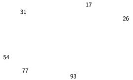
உருப்படி ஒவ்வொன்றிலும் சில வெளிப்படையான தகவல்களை நாம் பராமரிக்க முடிந்தால்,அதாவது அடுத்த உருப்படியின் இருப்பிடம், பின்னர் ஒவ்வொரு உருப்படிகளின் ஒப்பீட்டு நிலை போன்றவை ஆகவே ஒரு உருப்படியிலிருந்து அடுத்த உருப்படிக்கு இணைப்பைப் பின்பற்றுவதன் மூலம் வெளிப்படுத்தலாம்:
Relative positions maintained by explicit links

பட்டியலின் முதல் உருப்படியின் இருப்பிடம் வெளிப்படையாக குறிப்பிடப்பட வேண்டும் என்பதை கவனத்தில் கொள்ள வேண்டும். முதல் உருப்படி எங்கே என்று எங்களுக்கு தெரிந்தால் ,இரண்டாவது எங்கே என்று முதல் உருப்படி சொல்லும்.வெளி குறிப்பு பெரும்பாலும் பட்டியலின் head என குறிப்பிடப்படுகிறது. இதேபோல், அடுத்த உருப்படி இல்லை என்பதை கடைசி உருப்படி தெரிந்து கொள்ள வேண்டும்.
நுனி வகை - The Node Class
The basic building block for the linked list implementation is the node. Each node object must hold at least two pieces of information. First, the node must contain the list item itself. We will call this the data field of the node. In addition, each node must hold a reference to the next node. Here we provide one simple Python implementation:
class Node(object): def __init__(self, value): self.value = value self.next = None |
To construct a node, you need to supply the initial data value for the node. Evaluating the assignment statement below will yield a node object containing the value passed:
>>> temp = Node(93)
>>> temp.value
93
The special Python reference value None will play an important role in the Node class and later in the linked list itself. A reference to None will denote the fact that there is no next node. Note in the constructor that a node is initially created with next set to None. Since this is sometimes referred to as “grounding the node,” we will use the standard ground symbol to denote a reference that is referring to None. It is always a good idea to explicitly assign None to your initial next reference values.
A typical representation for a node
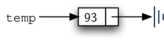
சீரற்ற பட்டியல் வகை - The Unordered List Class
As we suggested above, the unordered list will be built from a collection of nodes, each linked to the next by explicit references. As long as we know where to find the first node (containing the first item), each item after that can be found by successively following the next links. With this in mind, the UnorderedList class must maintain a reference to the first node. Below we show the constructor. Note that each list object will maintain a single reference to the head of the list.
class UnorderedList(object): def __init__(self): self.head = None |
Initially when we construct a list, there are no items. The assignment statement
>>> mylist = UnorderedList()
creates this linked list representation:
An empty list
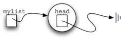
As we discussed in the Node class, the special reference None will again be used to state that the head of the list does not refer to anything. Eventually, the example list given earlier will be represented by this linked list:
A linked list of integers
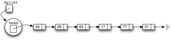
The head of the list refers to the first node which contains the first item of the list. In turn, that node holds a reference to the next node (the next item) and so on. It is important to note that the list class itself does not contain any node objects. Instead it contains a single reference to only the first node in the linked structure.
The is_empty method, shown below, simply checks to see if the head of the list is a reference to None. The result of the boolean expression self.head is None will only be true if there are no nodes in the linked list. Since a new list is empty, the constructor and the check for empty must be consistent with one another. This shows the advantage to using the reference None to denote the “end” of the linked structure. In Python, None can be compared to any reference. Two references are equal if they both refer to the same object. We will use this often in our remaining methods.
def is_empty(self): return self.head is None |
So, how do we get items into our list? We need to implement the add method. However, before we can do that, we need to address the important question of where in the linked list to place the new item. Since this list is unordered, the specific location of the new item with respect to the other items already in the list is not important. The new item can go anywhere. With that in mind, it makes sense to place the new item in the easiest location possible.
Recall that the linked list structure provides us with only one entry point, the head of the list. All of the other nodes can only be reached by accessing the first node and then following next links. This means that the easiest place to add the new node is right at the head, or beginning, of the list. In other words, we will make the new item the first item of the list and the existing items will need to be linked to this new first item so that they follow.
The linked list shown above was built by calling the add method a number of times.
>>> mylist.add(31)
>>> mylist.add(77)
>>> mylist.add(17)
>>> mylist.add(93)
>>> mylist.add(26)
>>> mylist.add(54)
Note that since 31 is the first item added to the list, it will eventually be the last node on the linked list as every other item is added ahead of it. Also, since 54 is the last item added, it will become the data value in the first node of the linked list.
The add method is shown below. Each item of the list must reside in a node object. We create a new node within the method and place the item as its value. Then we complete the process by linking the new node into the existing structure.
def add(self, item): temp = Node(item) temp.next = self.head self.head = temp |
This requires two steps as shown below. Step 1 (line 3) changes the next reference of the new node to refer to the old first node of the list. Now that the rest of the list has been properly attached to the new node, we can modify the head of the list to refer to the new node.
Adding a new node is a two-step process
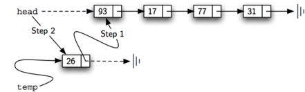
The order of the two steps described above is very important. What happens if the order of the steps is reversed? If the modification of the head of the list happens first, the result can be seen below. Since the head was the only external reference to the list nodes, all of the original nodes are lost and can no longer be accessed.
Result of reversing the order of the two steps
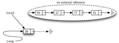
The next methods that we will implement–size, search, and remove–are all based on a technique known as linked list traversal. Traversal refers to the process of systematically visiting each node. To do this we use an external reference that starts at the first node in the list. As we visit each node, we move the reference to the next node by “traversing” the next reference.
To implement the size method, we need to traverse the linked list and keep a count of the number of nodes that occurred. Below we provide the Python code for counting the number of nodes in the list. The external reference is called current and is initialized to the head of the list in line 2. At the start of the process we have not seen any nodes so the count is set to 000. Lines 4–6 actually implement the traversal. As long as the current reference has not seen the end of the list (None), we move current along to the next node via the assignment statement in line 6. Every time current moves to a new node, we add 1 to count. Finally, count gets returned after the iteration stops.
def size(self): current = self.head count = 0 while current is not None: count = count + 1 current = current.next return count |
Searching for a value in a linked list implementation of an unordered list also uses the traversal technique. As we visit each node in the linked list we will ask whether the data stored there matches the item we are looking for. In this case, however, we may not have to traverse all the way to the end of the list. In fact, if we do get to the end of the list, that means that the item we are looking for must not be present. Also, if we do find the item, there is no need to continue.
Here is a possible implementation of search:
def search(self, item): current = self.head while current is not None: if current.value == item: return True current = current.next return False |
The remove method requires two logical steps. First, we need to traverse the list looking for the item we want to remove. Once we find the item (recall that we assume it is present), we must remove it. The first step is very similar to search. Starting with an external reference set to the head of the list, we traverse the links until we discover the item we are looking for. Since we assume that item is present, we know that the iteration will stop before current gets to None.
Once we have found the node to be removed, how do we remove it? One possibility would be to replace the value of the item with some marker that suggests that the item is no longer present. The problem with this approach is the number of nodes will no longer match the number of items. It would be much better to remove the item by removing the entire node.
In order to remove the node containing the item, we need to modify the link in the previous node so that it refers to the node that comes after current. Unfortunately, there is no way to go backward in the linked list. Since current refers to the node ahead of the node where we would like to make the change, it is too late to make the necessary modification.
The solution to this dilemma is to use two external references as we traverse down the linked list. current will behave just as it did before, marking the current location of the traverse. The new reference, which we will call previous, will always travel one node behind current. That way, when current stops at the node to be removed, previous will be referring to the proper place in the linked list for the modification.
Here is an implementation of a complete remove method:
def remove(self, item): current = self.head previous = None while True: if current.value == item: break previous, current = current, current.next if previous is None: self.head = current.next else: previous.next = current.next |
First we assign current and previous to the head of the list and None respectively. Then, on each iteration of our while loop, we break if current represents the node we wish to remove, and if not we update previous and current to current and current.next respectively. Again, the order of these two statements is crucial. previous must first be moved one node ahead to the location of current. At that point, current can be moved.
Here we illustrate the movement of previous and current as they progress down the list looking for the node containing the value 17:
"previous" and "current" move down the list
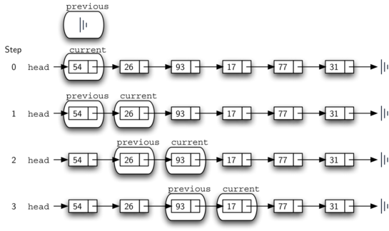
Once the searching step of the remove has been completed, we need to remove the node from the linked list. If previous is None, we know that current is in fact the head of the list, so we remove that node by updating the head of the list to the subsequent node, thereby losing the reference to the original head node:
Removing the first node from the list
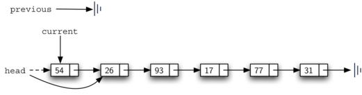
In all other cases, we know that both previous and current are nodes in the list, so we can remove current by setting the next attribute of previous to the node after current in the list:
Removing an item from the middle of the list
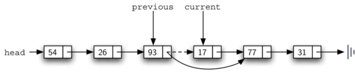
The remaining methods append, insert, index, and pop are left as exercises. Remember that each of these must take into account whether the change is taking place at the head of the list or someplace else. Also, insert, index, and pop require that we name the positions of the list. We will assume that position names are integers starting with 0.
5.3 சீரான பட்டியல் - Implementing an Ordered List
வரிசைப்படுத்தப்படட பட்டியலை செயல்படுத்த, சில அடிப்படை பண்புகளை அடிப்படையாகக் கொண்ட தொடர்பு நிலைகளை நங்கள் நினைவில்க் கொள்ள வேண்டும்.மேலே கொடுக்கப்பட்ட முழு எண்களின் பட்டியல் (17, 26, 31, 54, 77, மற்றும் 93) ஆனது கீழே காட்டப்பட்டுள்ளபடி இணைக்கப்பட்ட கட்டமைப்பால் குறிப்பிடப்பட முடியும்.மீண்டும், முனை மற்றும் இணைப்பு உருப்படிகளின் ஒப்பீட்டு நிலைப்பாட்டைக் குறிக்க இந்த அமைப்பு சிறந்தது.
An ordered linked list

OrderedList வகுப்பைச் செயல்படுத்த, முன்பு வரிசைப்படுத்தப்படாத பட்டியல்களுடன் காணப்பட்ட அதே நுட்பத்தைப் பயன்படுத்துவோம்.UnorderedList எனப்படும் துணை வகுப்பை உருவாக்குவதோடு __init__ முறையை மீண்டும் அப்படியே விட்டு விடுங்கள்,ஒரு வெற்று பட்டியல் இருக்கும் None என்பதற்கான head குறிப்பால் குறிக்கப்படுகிறது.
from unordered_list import Node, UnorderedList class OrderedList(UnorderedList): |
இணைக்கப்பட்ட பட்டியல் செயல்பாடுகளின் சிக்கலை திறனாய்வு செய்ய,அவற்றுக்கு இடையில் நகர்த்தல்கள் தேவை என்பதை நாங்கள் கருத்தில் கொள்ள வேண்டும். n முனைகள் உடைய ஒரு இணைக்கப்பட்ட பட்டியலைக் கவனியுங்கள். is_empty முறையானது O(1) ஆகும்.None என்பதற்கான தலை குறிப்பைச் சரிபார்க்க இதற்கு ஒரு படி தேவைப்படுகிறது.மறுபுறம் size இற்காக எப்பொழுதும் n படிகள் தேவைப்படுகிறது, ஏனெனில் எத்தனை முனைகள் தலையில் இருந்து இறுதி வரை செல்லாமல் இணைக்கப்பட்ட பட்டியலில் உள்ளன அறிய வழி இல்லை. எனவே,நீளம் என்பது O(n) ஆகும். வரிசைப்படுத்தப்படாத பட்டியலில் ஒரு பொருளைச் சேர்ப்பது எப்போதும் O(1) ஆக இருக்கும்.நாங்கள் இணைக்கப்பட்ட பட்டியலின் தலைப்பில் புதிய முனையை வைக்கின்றோம்.இருப்பினும், வரிசைப்படுத்தப்பட்ட பட்டியலுக்கு search மற்றும் remove, அத்தோடு add போன்றவற்றை செயற்படுத்த நகர்தல் செயற்பாடுகள் தேவை.இருந்த போதிலும் சராசரியாக பாதியளவு முனைகள் மட்டுமே நகர்த்தலுக்கு உள்ளாக்க வேண்டி இருக்கலாம்.இந்த முறைகள் அனைத்தும் O(n) இல் இருந்து மோசமான நிலையில் ஒவ்வொன்றும் பட்டியலில் உள்ள ஒவ்வொரு முனையையும் செயலாக்கும்.
பைதான் பட்டியல்களுக்கு முன்னர் கொடுக்கப்பட்ட உண்மையான செயல்திறனில் இருந்து இந்த செயல்பாட்டின் செயல்திறன் வேறுபடுகிறது என்பதை நீங்கள் கவனித்திருக்கலாம்.இந்த இணைக்கப்பட்ட பட்டியல்கள் பைதான் பட்டியல்கள் செயல்படுத்தப்படும் வழி அல்ல என்று அறிவுறுத்துகிறது.பைதான் பட்டியலின் உண்மையான செயல்படுத்தல் ஒரு கருத்தை அடிப்படையாகக் கொண்ட ஒரு வரிசையாகும்.இதைப் பற்றி பின்னர் விரிவாகப் பேசுவோம்.
Searching an ordered linked list
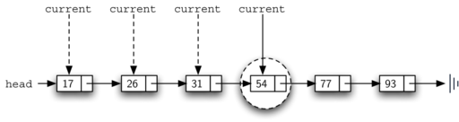
Below we provide an adaptation of the search method from our UnorderedList class to take advantage of this optimization.
def search(self, item): current = self.head while current is not None: if current.value == item: return True if current.value > item: return False current = current.next return False |
The most significant method modification will take place in add. Recall that for unordered lists, the add method could simply place a new node at the head of the list. It was the easiest point of access. Unfortunately, this will no longer work with ordered lists. It is now necessary that we discover the specific place where a new item belongs in the existing ordered list.
Assume we have the ordered list consisting of 17, 26, 54, 77, and 93 and we want to add the value 31. The add method must decide that the new item belongs between 26 and 54. Below we show the setup that we need. As we explained earlier, we need to traverse the linked list looking for the place where the new node will be added. We know we have found that place when either we run out of nodes (current becomes None) or the value of the current node becomes greater than the item we wish to add. In our example, seeing the value 54 causes us to stop.
Adding an item to an ordered linked list
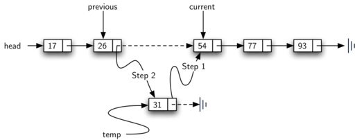
As we saw with unordered lists, it is necessary to have an additional reference, again called previous, since current will not provide access to the node that must be modified.
Once we have identified the position at which to add our new node, we construct it and place it correctly, either as the new head of the node (if previous is None) or between previous and current otherwise.
def add(self, item): current = self.head previous = None while current is not None: if current.value > item: break previous, current = current, current.next temp = Node(item) if previous is None: temp.next, self.head = self.head, temp else: temp.next, previous.next = current, temp |
We leave the remaining methods as exercises. You should carefully consider whether the unordered implementations will work given that the list is now ordered.
5.4 தொடர்பட்டியல் திறணாய்வு - Analysis of Linked Lists
இணைக்கப்பட்ட பட்டியல் செயல்பாடுகளின் சிக்கலை திறனாய்வு செய்ய,அவற்றுக்கு இடையில் நகர்த்தல்கள் தேவை என்பதை நாங்கள் கருத்தில் கொள்ள வேண்டும். n முனைகள் உடைய ஒரு இணைக்கப்பட்ட பட்டியலைக் கவனியுங்கள். is_empty முறையானது O(1) ஆகும். (None) என்பதற்கான தலை குறிப்பைச் சரிபார்க்க இதற்கு ஒரு படி தேவைப்படுகிறது.மறுபுறம் size இற்காக எப்பொழுதும் n படிகள் தேவைப்படுகிறது, ஏனெனில் எத்தனை முனைகள் தலையில் இருந்து இறுதி வரை செல்லாமல் இணைக்கப்பட்ட பட்டியலில் உள்ளன அறிய வழி இல்லை. எனவே,நீளம் என்பது O(n) ஆகும். வரிசைப்படுத்தப்படாத பட்டியலில் ஒரு பொருளைச் சேர்ப்பது எப்போதும் O(1) ஆக இருக்கும்.நாங்கள் இணைக்கப்பட்ட பட்டியலின் தலைப்பில் புதிய முனையை வைக்கின்றோம்.இருப்பினும், வரிசைப்படுத்தப்பட்ட பட்டியலுக்கு தேடல் (search) மற்றும் நீக்கல் (remove), அத்தோடு நுழைத்தல் (add) போன்றவற்றை செயற்படுத்த நகர்தல் செயற்பாடுகள் தேவை.இருந்த போதிலும் சராசரியாக பாதியளவு முனைகள் மட்டுமே நகர்த்தலுக்கு உள்ளாக்க வேண்டி இருக்கலாம்.இந்த முறைகள் அனைத்தும் O(n) இல் இருந்து மோசமான நிலையில் ஒவ்வொன்றும் பட்டியலில் உள்ள ஒவ்வொரு முனையையும் செயலாக்கும்.
பைதான் பட்டியல்களுக்கு முன்னர் கொடுக்கப்பட்ட உண்மையான செயல்திறனில் இருந்து இந்த செயல்பாட்டின் செயல்திறன் வேறுபடுகிறது என்பதை நீங்கள் கவனித்திருக்கலாம்.இந்த இணைக்கப்பட்ட பட்டியல்கள் பைதான் பட்டியல்கள் செயல்படுத்தப்படும் வழி அல்ல என்று அறிவுறுத்துகிறது.பைதான் பட்டியலின் உண்மையான செயல்படுத்தல் ஒரு கருத்தை அடிப்படையாகக் கொண்ட ஒரு வரிசையாகும்.இதைப் பற்றி பின்னர் விரிவாகப் பேசுவோம்.
6. அடுக்கு நிரல்படுத்தல் - Recursion
6.1 அடுக்கு நிரல்படுத்தல் அறிமுகம் - Introduction to Recursion
மறுபயன்பாடு என்பது சிக்கலைத் தீர்ப்பதற்கான ஒரு முறையாகும், இது ஒரு சிக்கலை சிறிய மற்றும் சிறிய துணைப் பிரச்சனைகளாகப் பிரிப்பதை உள்ளடக்கியது. கணினி அறிவியலில், மறுபயன்பாடு தன்னை தானே அழைக்கும் செயல்பாட்டை உள்ளடக்கியது. இது மேலோட்டமாகத் தோன்றாவிட்டாலும், மறுசீரமைப்பு சிக்கல்களுக்கு நேர்த்தியான தீர்வுகளை எழுத அனுமதிக்கிறது, இல்லையெனில் நிரலாக்கம் மிகவும் கடினமாக இருக்கும்.
6.2 எண் பட்டியலின் கூட்டுமதிப்பு - Calculating the Sum of a List of Numbers
We will begin our investigation with a simple problem that you already know how to solve without using recursion. Suppose that you want to calculate the sum of a list of numbers such as: [1,3,5,7,9][1, 3, 5, 7, 9][1,3,5,7,9]. An iterative function that computes the sum is shown below. The function uses an accumulator variable (total) to compute a running total of all the numbers in the list by starting with 000 and adding each number in the list.
def iterative_sum(numbers): total = 0 for n in numbers: total = total + n return total iterative_sum([1, 3, 5, 7, 9]) # => 2 |
Pretend for a minute that you do not have while loops or for loops. How would you compute the sum of a list of numbers? If you were a mathematician you might start by recalling that addition is a function that is defined for two parameters, a pair of numbers. To redefine the problem from adding a list to adding pairs of numbers, we could rewrite the list as a fully parenthesized expression. Such an expression looks like this:
((((1+3)+5)+7)+9) ((((1 + 3) + 5) + 7) + 9) ((((1+3)+5)+7)+9)
We can also parenthesize the expression the other way around,
(1+(3+(5+(7+9)))) (1 + (3 + (5 + (7 + 9)))) (1+(3+(5+(7+9))))
Notice that the innermost set of parentheses, (7+9)(7 + 9)(7+9), is a problem that we can solve without a loop or any special constructs. In fact, we can use the following sequence of simplifications to compute a final sum.
total= (1+(3+(5+(7+9)))) total = \ (1 + (3 + (5 + (7 + 9)))) total= (1+(3+(5+(7+9)))) total= (1+(3+(5+16))) total = \ (1 + (3 + (5 + 16))) total= (1+(3+(5+16))) total= (1+(3+21)) total = \ (1 + (3 + 21)) total= (1+(3+21)) total= (1+24) total = \ (1 + 24) total= (1+24) total= 25 |
How can we take this idea and turn it into a Python program? First, let’s restate the sum problem in terms of Python lists. We might say the the sum of the list numbers is the sum of the first element of the list (numbers[0]), and the sum of the numbers in the rest of the list (numbers[1:]). To state it in a functional form:
sumof(numbers)=first(numbers)+sumof(rest(numbers))
In this equation first(numbers) returns the first element of the list and rest(numbers) returns a list of everything but the first element. This is easily expressed in Python as:
def sum_of(numbers): if len(numbers) == 0: return 0 return numbers[0] + sum_of(numbers[1:]) sum_of([1, 3, 5, 7, 9]) # => 25 |
There are a few key ideas in this code sample to look at. First, on line 2 we are checking to see if the list is empty. This check is crucial and is our escape clause from the function. The sum of a list of length 0 is trivial; it is just zero. Second, on line 5 our function calls itself! This is the reason that we call the sum_of algorithm recursive. A recursive function is a function that calls itself.
The diagram below shows the series of recursive calls that are needed to sum the list [1,3,5,7,9]. You should think of this series of calls as a series of simplifications. Each time we make a recursive call we are solving a smaller problem, until we reach the point where the problem cannot get any smaller.
Series of recursive calls adding a list of numbers
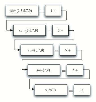
When we reach the point where the problem is as simple as it can get, we begin to piece together the solutions of each of the small problems until the initial problem is solved. The diagram below shows the additions that are performed as sum_of works its way backward through the series of calls. When sum_of returns from the topmost problem, we have the solution to the whole problem.
Series of recursive returns from adding a list of numbers
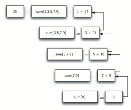
6.3 மூன்று விதிகள் - The Three Laws of Recursion
அசிமோவின் ரோபோக்களைப் போலவே, அனைத்து தொடர்ச்சியான வழிமுறைகளும் மூன்று முக்கியமான சட்டங்களுக்குக் கீழ்ப்படிய வேண்டும்:
- ஒரு சுழற்சி வழிமுறை ஒரு அடிப்படை வழக்கைக் கொண்டிருக்க வேண்டும்.
- ஒரு சுழற்சி வழிமுறை அதன் நிலையை மாற்றி அடிப்படை வழக்கை நோக்கி நகர வேண்டும்.
- ஒரு சுழற்சி வழிமுறை தன்னை தானே மீண்டும் மீண்டும் அழைக்க வேண்டும்.
இந்த சட்டங்கள் ஒவ்வொன்றையும் இன்னும் விரிவாகப் பார்ப்போம், அது sum_of ஆனது வழிமுறையில் எவ்வாறு பயன்படுத்தப்பட்டது என்பதைப் பார்ப்போம். முதலில், ஒரு அடிப்படை வழக்கு என்பது வழிமுறை மறுசீரமைப்பை நிறுத்த அனுமதிக்கும் நிபந்தனையாகும். ஒரு அடிப்படை வழக்கு என்பது பொதுவாக நேரடியாக தீர்க்கும் அளவுக்கு ஒரு சிறிய பிரச்சனையாகும் . sum_of ஆனது வழிமுறையில் அடிப்படை வழக்கு பட்டியலின் நீளம் 1 ஆகும்.
இரண்டாவது சட்டத்திற்கு கீழ்ப்படிய, அடிப்படை வழக்கை நோக்கி வழிமுறையை நகர்த்தும் நிலை மாற்றத்திற்கு நாம் ஏற்பாடு செய்ய வேண்டும்.நிலை மாற்றம் என்பது வழிமுறை பயன்படுத்தும் சில தரவு மாற்றியமைக்கப்பட்டது என்பதாகும்.பொதுவாக நம் பிரச்சனையை குறிக்கும் தரவு ஏதோ ஒரு வகையில் சிறியதாகிவிடும்.sum_of வழிமுறையில் எங்கள் முதன்மை தரவு அமைப்பு ஒரு பட்டியலாகும், எனவே பட்டியலில் நிலை மாற்றும் முயற்சிகளில் கவனம் செலுத்த வேண்டும்.அடிப்படை வழக்கு பட்டியல் நீளம் 1 என்பதால், அடிப்படை வழக்கை நோக்கிய இயற்கையான முன்னேற்றம் பட்டியலைக் குறைப்பதாகும். சுருக்க பட்டியலுடன் நாம் sum_of ஐ அழைக்கும் போது, sum_of வழிமுறையில் சரியாக நடக்கும்.
வழிமுறை தன்னை தானே அழைக்க வேண்டும் என்பதே இறுதிச் சட்டமாகும் . இது மீண்டும் மீண்டும் வருவதற்கான வரையறை. பலஆரம்பநிலை நிரலாளர்களுக்கு மறுபயன்பாடு ஒரு குழப்பமான கருத்து. ஒரு புதிய நிரலாளராக , செயல்பாடுகள் நல்லது என்பதை நீங்கள் கற்றுக்கொண்டீர்கள், ஏனென்றால் நீங்கள் ஒரு பெரிய பிரச்சனையை எடுத்து சிறிய பிரச்சனைகளாக உடைக்கலாம். ஒவ்வொரு பிரச்சினையையும் தீர்க்க ஒரு செயல்பாட்டை எழுதுவதன் மூலம் சிறிய சிக்கல்களை தீர்க்க முடியும். நாம் மறுசீரமைப்பைப் பற்றி பேசும்போது, நாம் வட்டங்களில் பேசிக்கொண்டிருப்பதாகத் தோன்றலாம். ஒரு செயல்பாட்டில் தீர்க்க எங்களுக்கு ஒரு சிக்கல் உள்ளது, ஆனால் அந்த செயல்பாடு தன்னை தானே அழைப்பதன் மூலம் சிக்கலை தீர்க்கிறது! ஆனால் தர்க்கம் வட்டமானது அல்ல; மறுசீரமைப்பின் தர்க்கம் ஒரு சிக்கலை சிறிய மற்றும் எளிதான பிரச்சனைகளாக உடைப்பதன் மூலம் தீர்க்கும் நேர்த்தியான வெளிப்பாடாகும்.
இந்த அத்தியாயத்தின் மீதமுள்ளவற்றில், சுழற்சிக்கான பல எடுத்துக்காட்டுகளைப் பார்ப்போம். ஒவ்வொரு நிகழ்விலும் மூன்று விதமான மறுசீரமைப்பைப் பயன்படுத்தி ஒரு பிரச்சனைக்கு ஒரு தீர்வை வடிவமைப்பதில் கவனம் செலுத்துவோம்.
6.4 எண்களை குறிப்பிட்ட தளத்திற்கு மாற்றுவது - Converting an Integer to Any Base
ஒரு முழு எண்ணை ஒரு சரமாக இரு அடி (Binary) எண்ணிற்கும் பதினாறு அடி எண்நிற்கும் இடையே ஒரு அடியை வைத்து மாற்ற வேண்டும் என வைத்துக் கொள்வோம்.எடுத்துக்காட்டாக, முழு எண் 10 ஐ தசமத்தில் அதன் சரம் பிரதிநிதித்துவமாக '10' ஆக அல்லது பைனரியில் அதன் சரம் பிரதிநிதித்துவத்தை '1010' ஆக மாற்றவும். இந்த சிக்கலை தீர்க்க பல வழிமுறைகள் இருந்தாலும், அடுக்குகள் அத்தியாயத்தில் விவாதிக்கப்பட்ட வழிமுறை உட்பட, பிரச்சனையின் தொடர்ச்சியான உருவாக்கம் மிகவும் நேர்த்தியானது.
அடி 10 மற்றும் எண் 769 ஐப் பயன்படுத்தி ஒரு உறுதியான உதாரணத்தைப் பார்ப்போம். CHAR_FOR_INT = '0123456789' போன்ற முதல் 10 இலக்கங்களுடன் தொடர்புடைய எழுத்துக்களின் வரிசை எங்களிடம் உள்ளது என்று வைத்துக்கொள்வோம்.10 -க்கும் குறைவான எண்ணை வரிசையில் பார்ப்பதன் மூலம் அதன் சரம் சமமானதாக மாற்றுவது எளிது. உதாரணமாக, எண் 9 ஆக இருந்தால், சரம் CHAR_FOR_INT [9] அல்லது '9' ஆகும். 769 என்ற எண்ணை 7, 6 மற்றும் 9 ஆகிய மூன்று ஒற்றை இலக்க எண்களாக பிரிக்க நாம் ஏற்பாடு செய்தால், அதை ஒரு சரமாக மாற்றுவது எளிது. 10 க்கும் குறைவான எண் ஒரு நல்ல அடிப்படை வழக்கு போல் தெரிகிறது.
எங்கள் அடிப்படை என்ன என்பதை அறிவது ஒட்டுமொத்த வழிமுறை மூன்று கூறுகளை உள்ளடக்கும் என்று பரிந்துரைக்கின்றது:
- ஒற்றை இலக்க எண்களின் தொடராக அசல் எண்ணைக் குறைக்கவும்
- தேடலைப் பயன்படுத்தி ஒற்றை இலக்க-எண்ணை ஒரு சரமாக மாற்றவும்.
- இறுதி இலக்கை உருவாக்க ஒற்றை இலக்க சரங்களை ஒன்றாக இணைக்கவும்.
அடுத்த கட்டம் நிலைமையை எவ்வாறு மாற்றுவது மற்றும் அடிப்படை வழக்கை நோக்கி முன்னேறுவது எப்படி என்பதைக் கண்டுபிடிப்பது. நாம் ஒரு முழு எண்ணுடன் வேலை செய்கிறோம் என்பதால், எந்த கணித செயல்பாடுகளால் ஒரு எண்ணைக் குறைக்கலாம் என்பதைக் கருத்தில் கொள்வோம். பெரும்பாலும் அவை பிரிவு மற்றும் கழித்தல் ஆகும் . கழித்தல் வேலை செய்யும்போது, நாம் எதைக் கழிக்க வேண்டும் என்பது தெளிவாகத் தெரியவில்லை. மீதமுள்ளவற்றுடன் முழு எண் பிரிவு நமக்கு தெளிவான திசையை அளிக்கிறது. நாம் மாற்ற முயற்சிக்கும் அடியினால் ஒரு எண்ணைப் பிரித்தால் என்ன ஆகும் என்று பார்ப்போம்.
769 ஐ 10 ஆல் வகுக்க முழு எண் வகுப்பைப் பயன்படுத்தி, மீதமுள்ள 9 உடன் 76 ஐப் பெறுகிறோம். இது எங்களுக்கு இரண்டு நல்ல முடிவுகளைத் தருகிறது. முதலில், எஞ்சியிருப்பது நமது தளத்தை விட குறைவான எண்ணிக்கையாகும், அதை உடனடியாக சரமாக மாற்றலாம். இரண்டாவதாக, நம் அசலை விட சிறியதாக இருக்கும் ஒரு எண்ணைப் பெறுகிறோம், மேலும் நமது அடித்தளத்தை விட ஒரு ஒற்றை எண் குறைவாக இருக்கும் அடிப்படை வழக்கை நோக்கி நம்மை நகர்த்துகிறது. இப்போது எங்கள் வேலை 76 ஐ அதன் சரம் பிரதிநிதித்துவமாக மாற்றுவதாகும். மீண்டும் 7 மற்றும் 6 இன் முடிவுகளைப் பெற முழு எண் பிரிவையும் மீதத்தையும் பயன்படுத்துவோம். இறுதியாக, 7 ஐ மாற்றுவதற்கான சிக்கலை நாங்கள் குறைத்துள்ளோம், இது n < அடித்தளத்தின் அடிப்படை வழக்கு நிலையை திருப்திப்படுத்துவதால், நாம் எளிதாக செய்ய முடியும், அங்கு அடிப்படை = 10. நாம் இப்போது செய்த தொடர் செயல்பாடுகள் கீழே விளக்கப்பட்டுள்ளன. நாம் நினைவில் கொள்ள விரும்பும் எண்கள் வரைபடத்தின் வலது பக்கத்தில் உள்ள மீதமுள்ள பெட்டிகளில் இருப்பதை கவனிக்கவும்.
Converting an integer to a string in base 10
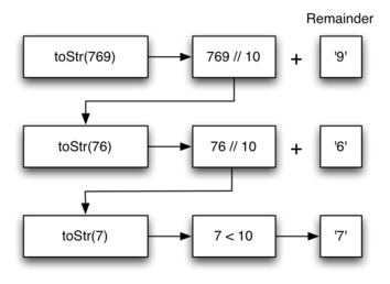
2 மற்றும் 16 க்கு இடையில் உள்ள எந்த தளத்திற்கும் இந்த வழிமுறையின் பைதான் செயல்படுத்தல் கீழே உள்ளது.
நாம் மாற்றும் அடித்தளத்தை விட n குறைவாக இருக்கும் அடிப்படை வழக்கை நாங்கள் சரிபார்க்கிறோம் என்பதை கவனிக்கவும். அடிப்படை வழக்கைக் கண்டறியும் போது, நாங்கள் மறுசீரமைப்பதை நிறுத்திவிட்டு, CHAR_FOR_INT வரிசையில் இருந்து சரத்தை திருப்பித் தருகிறோம். பின்னர் தொடர்ச்சியான அழைப்பு மற்றும் பிரிவைப் பயன்படுத்தி பிரச்சனையின் அளவைக் குறைப்பதன் மூலம் இரண்டாவது மற்றும் மூன்றாவது சட்டங்கள் இரண்டையும் நாங்கள் திருப்தி செய்கிறோம்.
வழிமுறையை மீண்டும் கண்டுபிடிப்போம்; இந்த முறை நாம் எண் 10 ஐ அதன் அடி 2 இனுடைய சர பிரதிநிதித்துவமாக மாற்றுவோம் ('1010').
கீழே உள்ள வரைபடம் நாம் தேடும் முடிவுகளைப் பெறுகிறது என்பதைக் காட்டுகிறது, ஆனால் இலக்கங்கள் தவறான வரிசையில் இருப்பது போல் தெரிகிறது.
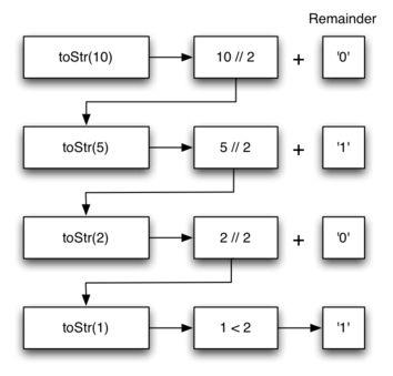
வழிமுறை சரியாக வேலை செய்கிறது, ஏனென்றால் நாங்கள் முதலில் திரும்ப திரும்ப அழைப்பு விடுக்கிறோம், பிறகு மீதமுள்ளவற்றின் சரம் பிரதிநிதித்துவத்தை சேர்க்கிறோம். நாங்கள் CHAR_FOR_INT இன் தேடலைத் மற்றும் to_string அழைப்பு ஆகியவற்றை செயற்படுத்தும் போது , இதன் விளைவாக வரும் சரம் பின்னோக்கி இருக்கும்! ஆனால் மறுசீரமைப்பு அழைப்பு திரும்பும்(call return ) வரை ஒருங்கிணைப்பு செயல்பாட்டை தாமதப்படுத்துவதன் மூலம், சரியான வரிசையில் முடிவைப் பெறுவோம். முந்தைய அத்தியாயத்தில் உள்ள அடுக்குகள் பற்றிய எங்கள் விவாதத்தை இது உங்களுக்கு நினைவூட்ட வேண்டும்.
CHAR_FOR_INT = '0123456789abcdef' def to_string(n, base): if n < base: return CHAR_FOR_INT[n] return to_string(n // base, base) + CHAR_FOR_INT[n % base] to_string(1453, 16) # => 5Ad |
Notice that we check for the base case where n is less than the base we are converting to. When we detect the base case, we stop recursing and simply return the string from the CHAR_FOR_INT sequence. Subsequently we satisfy both the second and third laws–by making the recursive call and by reducing the problem size–using division.
Let’s trace the algorithm again; this time we will convert the number 10 to its base 2 string representation ('1010').
The diagram below shows that we get the results we are looking for, but it looks like the digits are in the wrong order.
6.5 ஹனோய் கோபுரங்கள் - Tower of Hanoi
ஹனோய் புதிர் கோபுரத்தை 1883 ஆம் ஆண்டில் பிரெஞ்சு கணிதவியலாளர் எட்வார்ட் லூகாஸ் கண்டுபிடித்தார். இளம் பூசாரிகளுக்கு புதிர் வழங்கப்பட்ட ஒரு இந்து கோவிலின் புராணக்கதையால் அவர் ஈர்க்கப்பட்டார். காலத்தின் ஆரம்பத்தில், பூசாரிகளுக்கு மூன்று துருவங்கள் மற்றும் 64 தங்க வட்டுக்கள் அடுக்கி வைக்கப்பட்டன, ஒவ்வொன்றும் அதன் கீழே இருந்ததை விட சற்று சிறியதாக இருந்தது. இரண்டு முக்கிய தடைகளுடன், மூன்று துருவங்களில் இருந்து மற்றொன்றுக்கு அனைத்து 64 வட்டுகளையும் மாற்றுவதே அவர்களின் பணி. அவர்கள் ஒரு நேரத்தில் ஒரு வட்டை மட்டுமே நகர்த்த முடியும், மேலும் அவர்கள் ஒரு பெரிய வட்டை சிறிய ஒன்றின் மேல் வைக்க முடியாது. பூசாரிகள் மிகவும் திறமையாக வேலை செய்தனர், இரவும் பகலும், ஒவ்வொரு நொடியும் ஒரு வட்டு நகரும். அவர்கள் தங்கள் வேலையை முடித்ததும், கோவில் தூசிக்குள் சிதறிவிடும், உலகம் மறைந்துவிடும் என்று புராணக்கதை கூறுகிறது..
புராணக்கதை சுவாரஸ்யமாக இருந்தாலும், உலகம் எந்த நேரத்திலும் முடிவடையும் என்று நீங்கள் கவலைப்படத் தேவையில்லை. 64 வட்டுகளின் கோபுரத்தை சரியாக நகர்த்துவதற்கு தேவையான நகர்வுகளின் எண்ணிக்கை. 264−1 = 18,446,744,073,709,551,615 = 18,446,744,073,709,551,615264−1=18,446,744,073,709,551,615. ஒரு வினாடிக்கு ஒரு நகர்வு விகிதத்தில், அதாவது $$ 584,942,417,355 $$ ஆண்டுகள்! தெளிவாகவே இந்த புதிர் கண்ணில் பட்டதை விட அதிகமாக உள்ளது.
கீழே உள்ள அனிமேஷன் நான்கு டிஸ்க்குகளுடன் புதிருக்கு ஒரு தீர்வை நிரூபிக்கிறது. விதிகள் குறிப்பிடுவது போல், ஒவ்வொரு ஆப்பிலும் வட்டுகள் அடுக்கப்பட்டிருப்பதால், சிறிய வட்டுகள் எப்போதும் பெரிய வட்டுகளின் மேல் இருக்கும். இந்த புதிரை நீங்கள் இதற்கு முன் தீர்க்க முயற்சிக்கவில்லை என்றால், நீங்கள் இப்போது முயற்சி செய்ய வேண்டும். உங்களுக்கு ஆடம்பரமான வட்டுகள் மற்றும் துருவங்கள் தேவையில்லை - புத்தகங்கள் அல்லது காகிதத் துண்டுகளுடன் முயற்ச்சிக்கலாம்.
An animated solution of the Tower of Hanoi puzzle for four disks

இந்த சிக்கலை மீண்டும் மீண்டும் எப்படி தீர்க்க வேண்டும்? இந்த பிரச்சனையை எப்படி தீர்க்க போகிறீர்கள்? எங்கள் அடிப்படை வழக்கு என்ன? இந்த பிரச்சனையை கீழே இருந்து சிந்திக்கலாம். உங்களிடம் ஐந்து வட்டுகளின் கோபுரம் உள்ளது என்று வைத்துக்கொள்வோம், முதலில் பெக் ஒன்றில். நான்கு வட்டுகளின் கோபுரத்தை இரண்டாவது ஆப்புக்கு எப்படி மாற்றுவது என்பது உங்களுக்கு ஏற்கனவே தெரிந்திருந்தால், கீழே உள்ள வட்டை எளிதாக மூன்றாவது ஆப்புக்கு மாற்றலாம். ஆனால் உயரம் நான்கு உடைய கோபுரத்தை எப்படி நகர்த்துவது என்று தெரியாவிட்டால் என்ன செய்வது? மூன்று உயரம் கொண்ட கோபுரத்தை மூன்று இடங்களுக்கு நகர்த்துவது உங்களுக்குத் தெரியும் என்று வைத்துக்கொள்வோம். பின்னர் நான்காவது வட்டை இரண்டாவது ஆப்புக்கு நகர்த்தி அதன் மேல் உள்ள மூன்றை மூன்றிலிருந்து நகர்த்துவது எளிதாக இருக்கும். ஆனால் மூன்று உயரமுடைய கோபுரங்களை எப்படி நகர்த்துவது என்று தெரியாவிட்டால் என்ன செய்வது? இரண்டு வட்டுகளின் கோபுரத்தை இரண்டாகப் பிடுங்கி, மூன்றாவது வட்டை மூன்றாக ஆக்கி, அதன் மேல் இரண்டு உயரக் கோபுரத்தை நகர்த்துவது எப்படி? ஆனால் இதை எப்படி செய்வது என்று உங்களுக்கு இன்னும் தெரியாவிட்டால் என்ன செய்வது? ஒற்றை வட்டை மூன்றை ஆப்புக்கு நகர்த்துவது மிகவும் எளிதானது என்பதை நீங்கள் நிச்சயமாக ஒப்புக்கொள்வீர்கள், ஆனால் நீங்கள் இதை அற்பமானதாக கூறலாம். இது தயாரிப்பில் ஒரு அடிப்படை வழக்கு போல் தெரிகிறது.
ஒரு இடைநிலை துருவத்தைப் பயன்படுத்தி, ஒரு கோபுரத்தை தொடக்கத் துருவத்திலிருந்து, கோல் கம்பத்திற்கு எப்படி நகர்த்துவது என்பதற்கான உயர்மட்ட வரைவு இங்கே:
- இறுதி துருவத்தைப் பயன்படுத்தி உயரம் -1 கோபுரத்தை இடைநிலை துருவத்திற்கு நகர்த்தவும்.
- மீதமுள்ள வட்டை இறுதி துருவத்திற்கு நகர்த்தவும்.
- உயரம் -1 கோபுரத்தை இடைநிலை துருவத்திலிருந்து இறுதி துருவத்திற்கு அசல் துருவத்தைப் பயன்படுத்தி நகர்த்தவும்.
பெரிய வட்டுகள் அடுக்கின் அடிப்பகுதியில் இருக்கும் என்ற விதியை நாம் எப்போதும் கடைபிடிக்கும் வரை, மேலே உள்ள மூன்று படிகளையும் நாம் திரும்பத் திரும்பப் பயன்படுத்தலாம், எந்த பெரிய வட்டுகளும் கூட இல்லை என்றாலும் சிகிச்சை அளிக்கலாம். மேலே விபரிக்கப்பட்டதில் காணாமல் போன ஒரே விஷயம் ஒரு அடிப்படை வழக்கை அடையாளம் காண்பது. ஹனோய் பிரச்சனையின் எளிய கோபுரம் ஒரு வட்டின் கோபுரமாகும் . இந்த வழக்கில், நாம் ஒரு வட்டை மட்டுமே அதன் இறுதி இலக்குக்கு நகர்த்த வேண்டும். ஒரு வட்டின் கோபுரம் எங்கள் அடிப்படை வழக்காக இருக்கும். கூடுதலாக, மேலே விவரிக்கப்பட்டுள்ள படிகள் கோபுரத்தின் உயரத்தை 1 மற்றும் 3 ஆல் குறைப்பதன் மூலம் அடிப்படை வழக்கை நோக்கி நம்மை நகர்த்துகின்றன.
def move_tower(height, from_pole, to_pole, with_pole): if height >= 1: move_tower(height - 1, from_pole, with_pole, to_pole) move_disk(from_pole, to_pole) move_tower(height - 1, with_pole, to_pole, from_pole) |
மேலே உள்ள நிரல் தொகுப்பானது ஆங்கில விளக்கத்திற்கு கிட்டத்தட்ட ஒரே மாதிரியாக இருப்பதை கவனிக்கவும். வழிமுறையின் எளிமைக்கான திறவுகோல் என்னவென்றால், நாங்கள் இரண்டு வெவ்வேறு சுழற்சி அழைப்புகளைச் செய்கிறோம், முதலில் ஆரம்ப கோபுரத்தின் கீழ் வட்டை தவிர மற்ற அனைத்தையும் இடைநிலை துருவத்திற்கு நகர்த்துவோம். நாம் இரண்டாவது தொடர்ச்சியான அழைப்பைச் செய்வதற்கு முன், கீழே உள்ள வட்டை அதன் இறுதி ஓய்வு இடத்திற்கு நகர்த்துவோம். இறுதியாக இடைநிலை துருவத்திலிருந்து கோபுரத்தை மிகப்பெரிய வட்டின் மேல் நோக்கி நகர்த்துவோம். கோபுர உயரம் 0 ஆக இருக்கும்போது அடிப்படை வழக்கு கண்டறியப்பட்டது; இந்த வழக்கில் செய்ய எதுவும் இல்லை, எனவே move_tower செயல்பாடு வெறுமனே திரும்பும். அடிப்படை வழக்கை இந்த வழியில் கையாள்வது பற்றி நினைவில் கொள்ள வேண்டிய முக்கியமான விஷயம் என்னவென்றால், move_tower இல் இருந்து திரும்புவதே இறுதியாக move_disk செயல்பாட்டை அழைக்க அனுமதிக்கிறது.
நாங்கள் இந்த எளிய move_disk செயல்பாட்டை செயல்படுத்தினால், சிக்கலைத் தீர்க்க தேவையான நகர்வுகளை நாம் விளக்கலாம்:
def move_disk(from_pole, to_pole): print('moving disk from {} to {}'.format(from_pole, to_pole)) |
இப்போது, 3, 'A', 'B', 'C' வாதங்களுடன் move_tower ஐ அழைப்பது நமக்கு வெளியீட்டை வழங்கும்:
moving disk from A to B
moving disk from A to C
moving disk from B to C
moving disk from A to B
moving disk from C to A
moving disk from C to B
moving disk from A to B
இப்போது நீங்கள் move_tower மற்றும் move_disk இரண்டிற்குமான நிரலினைப் பார்த்திருக்கிறீர்கள், என்ன துருவங்களில் என்ன வட்டுகள் உள்ளன என்பதைத் தெளிவாகக் கண்காணிக்கும் தரவு அமைப்பு எங்களிடம் ஏன் இல்லை என்று நீங்கள் யோசிக்கலாம். இங்கே ஒரு குறிப்பு உள்ளது: நீங்கள் வட்டுகளை வெளிப்படையாகக் கண்காணிக்கப் போகிறீர்கள் என்றால், நீங்கள் ஒவ்வொரு துருவத்திற்கும் ஒன்று, மூன்று அடுக்கு பொருள்களைப் (stack objects ) பயன்படுத்தலாம். பதில் என்னவென்றால், பைத்தான் நமக்குத் தேவையான அடுக்குகளை மறைமுகமாக அழைப்பு அடுக்குகள் மூலம் வழங்குகிறது.
6.6 நிகழ்வு நிரலாக்கம் - Dynamic Programming
மாற்றமடையும் நிரலாக்கம் என்பது ஒரு குறிப்பிட்ட வகுப்பு பிரச்சனைகளைத் தீர்ப்பதற்கான ஒரு சக்திவாய்ந்த நுட்பமாகும், பொதுவாக அதனுடன் தொடர்புடைய சுழற்சி மூலோபாயத்தை விட மிகவும் திறமையான முறையில். குறிப்பாக, ஒரு பிரச்சனை "ஒன்றுடன் ஒன்று துணைப் பிரச்சனைகளை" கொண்டிருக்கும் போது, ஒரு தொடர்ச்சியான மூலோபாயம் தேவையற்ற கணக்கீட்டிற்கு வழிவகுக்கும். அதனுடன் தொடர்புடைய மாற்றமடையும் நிரலாக்க வியூகம் ஒன்றுடன் ஒன்று ஒன்றுடன் ஒன்று உப பிரச்சனைகளை நிவர்த்தி செய்து தீர்ப்பதன் மூலம் இத்தகைய தேவையற்றதுகளைத் தவிர்க்கலாம்.
சுருக்கத்தில் இந்த யோசனையைப் புரிந்து கொள்ள கடினமாக உள்ளது, எனவே ஒரு சில உதாரணங்களைக் கருத்தில் கொள்வோம்.
முதலில்,பிபனாச்சி எண்ணை திரும்பப் பெற ஒரு செயல்பாட்டை எழுதுவோம்: வரிசையில் $$ 0, 1 $$ தொடங்கி முந்தைய எண்களின் கூட்டுத்தொகையைக் கணக்கிடுவதன் மூலம் கட்டப்பட்டது n ஆவது எண் காட்டப்பட்ட்து.இதுபோல:
0,1,1,2,3,5,8,13,21...
பிபனாச்சி வரிசையில் நீங்கள் “மேலிருந்து கீழான” ஒரு அணுகுமுறையை எடுக்க முடியும் என்று உங்களுக்கு நன்கு தெரிந்திருக்கலாம்:பிபனாச்சி வரிசையின் மீள்செய்தல் தொடர்பை அடையாளம் காண்பதென்பது பிபனாச்சி வரிசையின் வரையறையை கருத்தில் கொள்வதன் மூலம் எளிய முறையில் சொல்லலாம்.வேறு வார்த்தைகளில் கூறுவதானால், "மேலிருந்து கீழ்" அணுகுமுறை "முந்தைய இரண்டு எண்களின் கூட்டுத்தொகையாக அடுத்தடுத்த எண்களைக் கணக்கிடுவது" என்ற அறிக்கையை கருதுகிறது மற்றும் தொடர்பு f(n)=f(n−1)+f(n−2).
எங்கள் அடிப்படை சந்தர்ப்பங்களாக 0 மற்றும் 1 இருப்பின் , இது நிரல் தொகுப்பை செயல்படுத்த வழிவகுக்கிறது, இது வரிசையின் கணித வரையறையைப் போல் தெரிகிறது:
def fib(n): if n <= 1: return n # base cases: return 0 or 1 if n is 0 or 1, respectively return fib(n - 1) + fib(n - 2) |
இது சரியான தீர்வாகும், ஆனால் இது fib(50) செயற்படுத்தி பதிலுக்காக காத்திருப்பவர்களுக்கு இது ஒரு சிக்கலை ஏற்படுத்துகிறது.மிக அதிக எண்ணிக்கையிலான தேவையற்ற தொடர்ச்சியான செயற்படுத்தல்கள் காரணமாக இந்த செயல்பாட்டின் இயக்க நேரம் O (2^n) ஆகும்.நாம் fib(n) ஐ அலைக்கும் போது நாம் fib(n - 1) மற்றும் fib(n - 2) மீண்டும் மீண்டும் அழைக்கின்றோம். அவை தங்களை (i) fib(n - 2) மற்றும் fib(n - 3); அத்தோடு (ii) fib(n - 3) மற்றும் fib(n - 4) மீண்டும் மீண்டும் அழைக்கின்றன.
சில தேவையற்ற அழைப்புகள் இருப்பதை நாங்கள் காணலாம், மேலும் அந்த தேவையற்ற அழைப்புகள் ஒவ்வொன்றும் முற்றிலும் தேவையற்ற அழைப்புகளின் மரங்களைத் தூண்டுகின்றன என்பதை நீங்கள் அடையாளம் காணலாம். fib(5) ஐ அழைப்பதற்க்கான மரத்தை வரைவதன் மூலம் இதை இன்னும் தெளிவாகக் காணலாம், நாம் கீழே செய்வது போல்:

fib(3) துணைமரம் முழுவதுமாக fib(4) துணை மரத்துக்கு கீழே நகல் செய்யப்பட்டுள்ளதையும் மற்றும் fib(2) துணைமரம் மூன்று முறை தோன்றியுள்ளதையும் நீங்கள் காணலாம்.n அதிகரிக்கும்போது, தேவையற்ற அழைப்புக்கான துணை மரங்களின் அளவு வியத்தகு அளவில் அதிகரிக்கிறது, அதே நேரத்தில் தனித்துவமான அழைப்புகளின் எண்ணிக்கை நேரியல்பாக மட்டுமே வளர்கிறது.வெறுமனே நாங்கள் தேவையான கணக்கீடுகளை மட்டுமே செய்வோம், எங்களுக்கு $$ 0 (n) $$ ஆனது இயங்கும் நேரத்தைக் கொடுக்கும்.
சுழல்நிலை சிக்கலைத் தீர்க்கும் "மேலிருந்து கீழ்" அணுகுமுறைக்கு ஒரு எதிராக , மாறும் நிரலாக்கத்தின் ஆச்சரியமில்லாத "கீழ்நோக்கி" அணுகுமுறை இருப்பதைக் கருத்தில் கொள்ள இது ஒரு நல்ல நேரம்.
இந்த பிரச்சனைக்கு மாறும் நிரலாக்கத்தினைப் பயன்படுத்துவதன் மூலம், "0 மற்றும் 1 இல் தொடங்கி, f (n) க்கு ஒரு பதிலை எவ்வாறு உருவாக்குவது?" எங்களை நாங்களே கேட்க முடியும்.n ஆனது 0 அல்லது 1 ஆக இருந்தால், நாங்கள் உடனடியாக பதிலளிக்க முடியும். இருப்பினும், அது 2 ஆக இருந்தால், 1 என்ற பதிலைத் தீர்மானிக்க 0 மற்றும் 1 ஐ சேர்க்க வேண்டும். n ஆனது 3 ஆக இருந்தால், நாம் இப்போது தீர்மானித்த f (2) க்கு பதிலைச் சேர்க்க வேண்டும். முன்னர் நிர்ணயிக்கப்பட்டது 1 ஆகவே மொத்தம் 2 ஆகும். இந்த மூலோபாயத்தைப் பின்பற்றி,எங்கள் n க்கான பதிலை அடையும் வரை, 3, 5, 8, என்று பதிலைப் பெறுகிறோம்.
எந்த நேரத்திலும் நாம் முந்தைய இரண்டு கணக்கீடுகளின் நினைவகத்தை மட்டுமே தக்க வைத்துக் கொள்ள வேண்டும், நாம் எப்போதும் அதே தொகையை இருமுறை பெறுவதில்லை.
இந்த மூலோபாயத்தை செயல்படுத்துவது இதுபோல் தோன்றலாம்:
def fib(n): a, b = 0, 1 for _ in range(n): a, b = a + b, a return a |
இதைச் செயல்படுத்துவதன் மூலம், எங்கள் தொடர்ச்சியான தீர்வின் சில நேர்த்தியையும் வாசிப்பையும் தியாகம் செய்கிறோம், ஆனால் மிகச் சிறந்த O (n) இயங்கும் நேரத்தையும் O (1) இடச் செலவையும் பெறுகிறோம்.
தொடர்ச்சியான மற்றும் மாறும் நிரலாக்க அணுகுமுறைகள் கண்டுபிடிக்க இன்னும் கொஞ்சம் வேலை தேவைப்படும் ஒரு சிக்கலை இப்போது கருத்தில் கொள்வோம்.
உயரம் H மற்றும் அகலம் W உடைய பின்னல் தட்டி கொடுக்கப்பட்டால், மேல் இடது மூலையில் இருந்து கீழ் வலது மூலை வரை எத்தனை தனித்துவமான குறுகிய பாதைகள் உள்ளன ?
உதாரணமாக, உயரம் மற்றும் அகலம் 2 ஐ கொண்ட பின்னல் தட்டினைக் கவனியுங்கள்:
மேல் இடதிலிருந்து கீழ் வலதுபுறம் வரை உள்ள குறுகிய பாதை நீளம் 4 ஆக இருப்பதையும், நீளம் 4 ஆக 6 தனித்துவமான பாதைகள் இருப்பதையும் நாம் காணலாம்:
இந்த சிக்கலை ஆராய்ந்து, எந்தவொரு குறுகிய பாதையும் எப்போதும் கீழ்நோக்கி மற்றும் வலதுபுறமாக முன்னேற வேண்டும் என்பதை நாங்கள் உணர்கிறோம் - எந்த இடத்திலும் மேலே முன்னேறும் அல்லது இடதுபுறமாக செல்லும் எந்தப் பாதையும் "குறுகியதாக" இருக்க வாய்ப்பில்லை. மேலும் ஆராய்ந்து, சரியான பாதையில் தொடங்கும் பாதைகள் (மேலே உள்ள மேல் வரியில் காட்டப்பட்டுள்ளது) மற்றும் கீழ்நோக்கி (கீழே கீழ் வரியில் காட்டப்பட்டுள்ளது) தொடங்கும் பாதைகளை குழுவாக்குவதன் மூலம், இந்த பயணப்படும் பிரச்சனையை உப பிரச்சனைகளாக உடைக்கலாம்.
இந்த சிக்கலை ஆராய்ந்து, எந்தவொரு குறுகிய பாதையும் எப்போதும் கீழ்நோக்கி மற்றும் வலதுபுறமாக முன்னேற வேண்டும் என்பதை நாங்கள் உணர்கிறோம் - எந்த இடத்திலும் மேலே முன்னேறும் அல்லது இடதுபுறமாக செல்லும் எந்தப் பாதையும் "குறுகியதாக" இருக்க வாய்ப்பில்லை. மேலும் ஆராய்ந்து, சரியான பாதையில் தொடங்கும் பாதைகள் (மேலே உள்ள மேல் வரியில் காட்டப்பட்டுள்ளது) மற்றும் கீழ்நோக்கி (கீழே கீழ் வரியில் காட்டப்பட்டுள்ளது) தொடங்கும் பாதைகளை குழுவாக்குவதன் மூலம், இந்த பயணப்படும் பிரச்சனையை உப பிரச்சனைகளாக உடைக்கலாம்.
குறிப்பாக,மொத்த பாதைகளின் எண்ணிக்கையானது பின்னல் தட்டியின் H×W இல் தங்கியிருக்கும்.அது (H - 1) ×W மற்றும் H × (W - 1) இன் கூட்டுத்தொகையாகும்.
எங்கள் 2×2 உதாரணத்துடன் தொடரும், சரியான படி தொடங்கும் பாதைகள், 1 x 2 துணைப் பிரச்சனைக்கு இந்த மூன்று தீர்வுகளுடன் வழிவகுக்கிறது:
உற்று நோக்கினால், இதை நாங்கள் 2 x 2 பிரச்சனைக்கு நமது முதல் மூன்று தீர்வுகளின் வலது புறப் பகுதியை மீண்டும் மீண்டும் பார்க்கிறோம்.
இதேபோல், எங்கள் 2 x 2 பிரச்சனையில் கீழ்நோக்கி தொடங்கும் பாதைகள் 2 x 1 துணைப் பிரச்சனைக்கு பின்வரும் மூன்று தீர்வுகளுடன் வழிவகுக்கிறது:
இந்த முறை நெருக்கமாகப் பார்த்தால், இது 2 x 2 பிரச்சனைக்கு எங்கள் இறுதி மூன்று தீர்வுகளின் கீழ் பகுதி மீண்டும் மீண்டும் வருவதைக் காண்கிறோம்.
H x W பின்னல் தட்டியின் மொத்த பாதைகளின் எண்ணிக்கை ஒரு (H - 1) x W பின்னல் தட்டி மற்றும் H x (W - 1) பின்னல் தட்டிஆகியவற்றின் கூட்டுத்தொகை என்று நாம் சிறிது நம்பிக்கையுடன் கூறலாம். பிரச்சனையின் தொடர்ச்சியான தன்மையை ஆராய மேல்நோக்கி அணுகுவதன் மூலம், ஒரு சுழற்சி தொடர்பை நாங்கள் அடையாளம் கண்டுள்ளோம்: f(h, w) = f(h, w - 1) + f(w, h - 1).
பிரச்சனைக்கு ஒரு தொடர்ச்சியான தீர்வை எழுதுவதற்கு முன், நாம் அடிப்படை வழக்கையும் அங்கீகரிக்க வேண்டும்: நமது உப பிரச்சனையின் h அல்லது w என்பது 0 ஆயின் நாம் ஒரு நேர் கோட்டைக் கையாளுகின்றோம் , எனவே பாதைகளின் எண்ணிக்கை வெறுமனே 1 ஆகும்
எங்கள் அடிப்படை வழக்கு மற்றும் பொது வழக்கை ஒன்றாக சேர்த்து, ஒரு சுருக்கமான சுழற்சி தீர்வைப் பெறுகிறோம்:
def num_paths(height, width): if height == 0 or width == 0: return 1 return num_paths(height, width - 1) + num_paths(height - 1, width) |
துரதிருஷ்டவசமாக, எங்களது ஒன்றுடன் ஒன்று மேற்பொருந்துதல் துணைப் பிரச்சனைகளில் தேவையற்ற அழைப்புகள் காரணமாக மற்றொரு O (2n) தீர்வை (n = H + W) கொண்டுள்ளோம். உதாரணமாக, f(3,2)கணக்கிடுவதில் f(2,2) மற்றும் f(3,1) ஆகியவற்றைக் கணக்கிடுவது அடங்கும், ஆனால் பின்னர் f(2,3)கணக்கிடுவதில் நாம் தேவையற்ற முறையில் f(2,2) ஐ மீண்டும் ஒரு முறை அழைக்கிறோம்.
ஓடும் நேரம் O (2n) என்பதை உங்களை நம்ப வைக்க num_paths(2, 2) என்ற அழைப்பு மரத்தை கருத்தில் கொள்ளுங்கள்:

மீண்டும் இது நமக்கு ஒரு சமிக்ஞையாக இருக்க வேண்டும், முக்கிய பிரச்சனைக்கு தீர்வு காண்பதற்கு முன், உப பிரச்சனைகளுக்கான பதிலை கணக்கிட்டு, சேமித்து வைப்பதன் மூலம் வேகமான தீர்வை நாம் கண்டுபிடிக்க முடியும்.
பிரச்சனையின் சில ஆய்வுகளுக்குப் பிறகு, பின்னல் தட்டியில் உள்ள எந்தப் புள்ளிக்கும் தனித்துவமான பாதைகளின் எண்ணிக்கையைக் கணக்கிடுவதற்கு, இடதுபுறம் மற்றும் கேள்வியில் மேலே உள்ள ஒவ்வொரு புள்ளிகளுக்கும் பாதைகளின் எண்ணிக்கையின் துணைப் பிரச்சினைகளை நாங்கள் தீர்க்க வேண்டும் என்பதை நீங்கள் உணரலாம்.இதையொட்டி, ஒவ்வொரு புள்ளிகளுக்கும் இடதுபுறம் மற்றும் அந்த புள்ளிகளுக்கு மேலே உள்ள பாதைகளின் எண்ணிக்கையின் துணைப் பிரச்சனைகளுக்கு முதலில் பதிலளித்தால் அந்த உப பிரச்சனைகள் தீர்க்கப்படும்.தர்க்கரீதியான முடிவு என்னவென்றால், நாம் மேல் இடது முனையிலிருந்து தொடங்கினால் (இதை நாம் 1 வழியில் மட்டுமே அடைய முடியும் என்று சொல்லலாம்) பிறகு நாம் ஒவ்வொரு கட்டத்திலும்,ஒவ்வொரு வரிசை வரிசையாக திரும்பவும், எனவே அந்த இடத்திற்கான பாதைகளை கணக்கிடலாம். மேலே உள்ள இடங்கள் மற்றும் இடதுபுறம் உள்ள பாதைகளின் கூட்டுத்தொகை, நமது மறு செய்கையின் தன்மையால் நாம் ஏற்கனவே ஒரு முறை துல்லியமாக கணக்கிட்டுள்ளோம்.
நாங்கள் தொடரும்போது எங்கள் கணக்கிடப்பட்ட மதிப்புகளை சேமிக்க பட்டியல்களின் பட்டியலைப் பயன்படுத்தலாம். H x W பின்னல் தட்டிக்கு , நாம் ஒரு (H + 1) x (W + 1) பட்டியல்களின் பட்டியலைப் பயன்படுத்தலாம், ஒவ்வொரு நுழைவும் அந்த உச்சியை அடைய ஒருவர் எடுக்கக்கூடிய பாதைகளின் எண்ணிக்கையைக் குறிக்கும். மேல் அல்லது இடது விளிம்புகளில் ஒரு உச்சியை அடைய ஒரே ஒரு வழி இருக்கிறது என்று நமக்குத் தெரியும் என்பதால், மதிப்புகளை 1 க்கு ஆரம்பிக்கலாம். பின்னர், ஒவ்வொரு வரிசையின் ஒவ்வொரு நுழைவு வழியாகவும், மேலே மற்றும் இடதுபுறத்தில் உள்ள உச்சநிலைகளுக்கு பாதைகளின் எண்ணிக்கையைச் சேர்ப்பதன் மூலம் அந்த உச்சத்தின் பாதைகளின் எண்ணிக்கையை நாம் தீர்மானிக்க முடியும். இறுதியாக, எங்கள் குறிப்பாணையின்(memo) கடைசி வரிசையின் கடைசி உள்ளீட்டில் கணக்கிடப்பட்ட மதிப்பை நாங்கள் அணுகுகிறோம், இது முழு பின்னல் தட்டியையும் கடந்து செல்லும் பாதைகளின் எண்ணிக்கையைக் குறிக்கிறது.
உதாரணமாக, இந்த உத்தியைப் பயன்படுத்தி f(2, 2) கணக்கிடும் செயல்பாட்டில் நாம் உருவாக்கும் குறிப்பு இது:
[
[1, 1, 1],
[1, 2, 3],
[1, 3, 6]
]
மீண்டும் நாங்கள் எங்கள் பதிலுக்கு வருகிறோம் அது 6.
f(10, 10) க்கான குறிப்பு இதுபோல் தெரிகிறது:
[
[1, 1, 1, 1, 1, 1, 1, 1, 1, 1, 1],
[1, 2, 3, 4, 5, 6, 7, 8, 9, 10, 11],
[1, 3, 6, 10, 15, 21, 28, 36, 45, 55, 66],
[1, 4, 10, 20, 35, 56, 84, 120, 165, 220, 286],
[1, 5, 15, 35, 70, 126, 210, 330, 495, 715, 1001],
[1, 6, 21, 56, 126, 252, 462, 792, 1287, 2002, 3003],
[1, 7, 28, 84, 210, 462, 924, 1716, 3003, 5005, 8008],
[1, 8, 36, 120, 330, 792, 1716, 3432, 6435, 11440, 19448],
[1, 9, 45, 165, 495, 1287, 3003, 6435, 12870, 24310, 43758],
[1, 10, 55, 220, 715, 2002, 5005, 11440, 24310, 48620, 92378],
[1, 11, 66, 286, 1001, 3003, 8008, 19448, 43758, 92378, 184756]
]
நாம் விவாதித்த மாறும் நிரலாக்க உத்தியின் சாத்தியமான செயல்படுத்தல் கீழே உள்ளது:
def num_paths_dp(height, width): memo = [[1] * (width + 1) for _ in range(0, height + 1)] for i, row in enumerate(memo): for j, _ in enumerate(row): if i == 0 or j == 0: continue memo[i][j] = memo[i - 1][j] + memo[i][j - 1] return memo[-1][-1] |
இந்த செயல்பாட்டிற்கான நேரம் மற்றும் இடச் செலவு இரண்டும் O(H×W) ஆகும்,முந்தைய நேரம்
O(2{H + W}) மற்றும் O (H + W) இடம் ஆகியவற்றை ஒப்பிடும்போது,H மற்றும் W என்பன அதிகரிக்கும் போது பெரிய மடங்கு வித்தியாசத்தை உருவாக்குகிறது.
குறிப்பாக நினைவக இடம் பற்றி கவலையாக இருந்தால், இடச் செலவை முந்தைய வரிசையின் குறிப்பை மட்டும் தக்கவைத்துக்கொள்வதன் மூலம் O(W) இற்கு குறைக்கலாம்.இது வாசிப்பவரின் பயிற்சிக்காக விடப்படுகின்றது.
6.7 அடுக்கு நிரலாக்கத்தை செயற்படுத்தல் - Implementing Recursion
கீழ்கண்ட நிரலில் 'CHAR_FROM_INT' இலிருந்து சாரமொன்றிற்காக to_string இன் தொடர்ச்சியான அழைப்பின் முடிவை இணைப்பதற்குப் பதிலாக,தொடர்ச்சியான அழைப்பைச் செய்வதற்கு முன் சரங்களை ஒரு அடுக்கில் தள்ள எங்கள் வழிமுறையை மாற்றினோம். இந்த மாற்றியமைக்கப்பட்ட வழிமுறையின் நிரல் தொகுப்பு இப்படி இருக்கலாம்:
CHAR_FROM_INT = '0123456789ABCDEF' def to_string(n,base): stack = [] while n > 0: if n < base: stack.append(CHAR_FROM_INT[n]) else: stack.append(CHAR_FROM_INT[n % base]) n = n // base result = '' while stack: result = result + stack.pop() return result to_string(1453,16) # => 5AD |
ஒவ்வொரு முறையும் நாம் to_string க்கு அழைப்பு விடுக்கும்போது, அடுக்கில் ஒரு குறியுருவை தள்ளுவோம். முந்தைய எடுத்துக்காட்டுக்குத் திரும்புகையில், to_string இற்கான நான்காவது அழைப்பிற்குப் பிறகு அடுக்கானது கீழே உள்ள வரைபடத்தைப் போல் இருக்கும் . இப்போது நாம் குறியிருக்களை இலகுவாக வெளியே எடுக்கவும் மற்றும் அவற்றை இறுதி முடிவான '1010' இல் இணைக்க முடியும்.
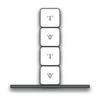
முந்தைய உதாரணம் பைதான் எவ்வாறு ஒரு சுழற்சி செயல்பாட்டு அழைப்பை செயல்படுத்துகிறது என்பதைப் பற்றிய சில நுண்ணறிவுகளை நமக்கு அளிக்கிறது. பைத்தானில் ஒரு செயல்பாடு அழைக்கப்படும் போது, செயல்பாட்டின் உள்ளூர் மாறிகளைக் கையாள ஒரு அடுக்கு சட்டகம் ஒதுக்கப்படுகிறது. செயல்பாடு திரும்பும்போது, அழைப்பு செயல்பாட்டை அணுகுவதற்காக திரும்பும் மதிப்பு அடுக்கின் மேல் விடப்படும். கீழேயுள்ள வரைபடம் அழைப்பு அடுக்கை அறிக்கை திரும்பலுக்கு (statement return) பிறகு விளக்குகிறது.
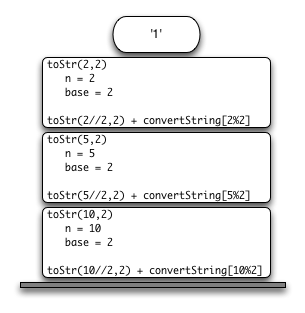
அடுக்கில் to_string(2 // 2, 2) க்கான அழைப்பு '1' இனை திரும்பும் மதிப்பாக (return value ) விட்டுச்செல்கிறது என்பதை கவனிக்கவும். '1' + CHAR_FROM_INT[2 % 2] என்ற சமன்பாட்டில் செயற்பாட்டின் அழைப்பு (to_string(1,2)) க்குப் பதிலாக இந்த திரும்பும் மதிப்பு பயன்படுத்தப்படுகிற
து, இது அடுக்கில் '10' என்ற சரத்தை விட்டுச்செல்லும்.இந்த வழியில், மேலே உள்ள எங்கள் வழிமுறையில் நாம் வெளிப்படையாகப் பயன்படுத்திய அடுக்கின் இடத்தை பைதானின் அழைப்பு அடுக்கு எடுக்கிறது.எங்கள் பட்டியலில் சுருக்கமான உதாரணமாக , குவிப்பான் மாறியின் இடத்தைப் பெறும் அடுக்கில் திரும்பும் மதிப்பைப் பற்றி நீங்கள் சிந்திக்கலாம்.
அடுக்கு சட்டகமானது செயல்பாட்டால் பயன்படுத்தப்படும் மாறிகளுக்கு ஒரு வாய்ப்பை வழங்குகிறது. நாங்கள் ஒரே செயல்பாட்டை மீண்டும் மீண்டும் அழைத்தாலும், ஒவ்வொரு அழைப்பும் செயல்பாட்டிற்கு உள்ளூர் மாறிகளுக்கு ஒரு புதிய நோக்கத்தை உருவாக்குகிறது.
7. தேடல் அல்கோரிதங்கள் - Searching
7.1 தேடல் - Searching
இந்த பிரிவில் நாம் தேடுதலைப் படிப்போம். தேடுதல் என்பது உருப்படிகளின் தொகுப்பில் ஒரு குறிப்பிட்ட உருப்படியைக் கண்டுபிடிப்பதற்கான வழிமுறையாகும். உருப்படி இருக்கிறதா என்று ஒரு தேடல் பொதுவாக True அல்லது False என்று பதிலளிக்கிறது. சில சமயங்களில் உருப்படியைக் கண்டறிந்த இடத்திற்குத் திரும்ப மாற்றியமைக்கலாம். இங்குள்ள எங்கள் நோக்கங்களுக்காக, நாங்கள் உறுப்பினர் பற்றிய கேள்வியில் நாங்கள் கவனம் செலுத்துவோம்.
பைத்தானில், ஒரு உருப்படி உருப்படிகளின் பட்டியலில் இருக்கிறதா என்று கேட்க மிகவும் எளிதான வழி உள்ளது. நாங்கள் in இயக்கியை (operator) பயன்படுத்துகிறோம்.
>>> 15 in [3, 5, 2, 4, 1]
False
>>> 3 in [3, 5, 2, 4, 1]
True
பைத்தானில் ஒரு தேடலை எளிதாக நடத்துவதால், தேடலை ஒரு படிமுறைப் பிரச்சினையாகப் படிப்பதன் நோக்கம் என்ன என்று நீங்கள் யோசிக்கலாம். விரைவான தேடலுக்காக வடிவமைக்கப்பட்ட தரவு கட்டமைப்புகள் மற்றும் குறிப்பாக தரவுத்தளங்கள் போன்ற வேறு எங்கும் எழும் என்பதால் தேடலை இயக்குவதற்குப் பயன்படுத்தப்படும் அடிப்படை செயல்முறை புரிந்து கொள்ள வேண்டியது முக்கியம்.
ஒரு தொகுப்பில் ஒரு பொருளைத் தேட பல வழிகள் உள்ளன என்று மாறிவிடும். இதுபோன்ற இரண்டு வழிகளுக்கு இடையேயான வித்தியாசத்தில் நாங்கள் இங்கே கவனம் செலுத்துகிறோம் - தொடர்ச்சியான தேடல் மற்றும் இரும நிலைத் தேடல்.
7.2 வரிசைபடுத்தப்பட்ட தேடல் - Sequential Search
ஒரு பட்டியல் போன்ற ஒரு தொகுப்பில் தரவு உருப்படிகள் சேமிக்கப்படும் போது, அவை ஒரு நேர்கோட்டு அல்லது தொடர்ச்சியான தொடர்பைக் கொண்டிருப்பதாகச் சொல்கிறோம். ஒவ்வொரு தரவு உருப்படியும் மற்றவற்றுடன் தொடர்புடைய நிலையில் சேமிக்கப்படுகிறது. பைதான் பட்டியல்களில், இந்த தொடர்பு நிலைகள் தனிப்பட்ட உருப்படிகளின் குறியீட்டு மதிப்புகள் ஆகும். இந்த குறியீட்டு மதிப்புகள் வரிசைப்படுத்தப்பட்டிருப்பதால், அவற்றை நாம் வரிசையாகப் பார்க்க முடியும். இந்த செயல்முறை எங்கள் முதல் தேடுதல் நுட்பமான தொடர்ச்சியான தேடலுக்கு வழிவகுக்கிறது.
கீழே உள்ள வரைபடம் இந்த தேடல் எவ்வாறு செயல்படுகிறது என்பதைக் காட்டுகிறது. பட்டியலில் முதல் உருப்படியிலிருந்து தொடங்கி, நாம் எதைத் தேடுகிறோம் என்பதைக் கண்டுபிடிக்கும் வரை அல்லது உருப்படிகள் தீரும் வரை, தொடர்ச்சியான வரிசைமுறையைப் பின்பற்றி, உருப்படியிலிருந்து உருப்படிக்கு நகர்கிறோம். எங்களிடம் உருப்படிகள் தீர்ந்து விட்டால், நாங்கள் தேடும் உருப்படி இல்லை என்று கண்டுபிடித்துள்ளோம்.
Sequential search of a list of integers
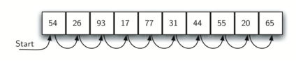
இந்த வழிமுறைகளுக்கான பைதான் செயல்படுத்தல் கீழே காட்டப்பட்டுள்ளது. செயல்பாட்டிற்கு பட்டியல் மற்றும் நாம் தேடும் உருப்படி தேவை மற்றும் அது இருக்கிறதா என்று பூலியன் மதிப்பை வழங்குகிறது. இந்த நோக்கத்திற்காக நாங்கள் பைத்தானின் in இயக்கியை பயன்படுத்துவோம் என்பதை நினைவில் கொள்ளுங்கள், எனவே கீழே உள்ள வழிமுறையை எங்களுக்கு வழங்காவிட்டால் நாங்கள் என்ன செய்வோம் என்று நீங்கள் சிந்திக்கலாம்.
def sequential_search(alist, item): position = 0 while position < len(alist): if alist[position] == item: return True position = position + 1 return False testlist = [1, 2, 32, 8, 17, 19, 42, 13, 0] sequential_search(testlist, 3) # => False sequential_search(testlist, 13) # => True |
தொடர்ச்சியான தேடலின் திறனாய்வு - Analysis of Sequential Search
தேடல் வழிமுறைகளை திறனாய்வு செய்ய, கணக்கீட்டின் அடிப்படை அலகு பற்றி நாம் முடிவு செய்ய வேண்டும். சிக்கலைத் தீர்க்க இது மீண்டும் மீண்டும் செய்யப்பட வேண்டிய பொதுவான படி என்பதை நினைவில் கொள்ளுங்கள். தேடலுக்கு, நிகழ்த்தப்பட்ட ஒப்பீடுகளின் எண்ணிக்கையை எண்ணுவது அர்த்தமுள்ளதாக இருக்கிறது. ஒவ்வொரு ஒப்பீடும் நாம் தேடும் உருப்படியைக் கண்டறியலாம் அல்லது கண்டுபிடிக்காமல் இருக்கலாம். கூடுதலாக, நாங்கள் இங்கே மற்றொரு அனுமானத்தை செய்கிறோம். உருப்படிகளின் பட்டியல் எந்த வகையிலும் வரிசைப்படுத்தப்படவில்லை . உருப்படிகள் தோராயமாக பட்டியலில் சேர்க்கப்பட்டுள்ளன. வேறு வார்த்தைகளில் கூறுவதானால், நாம் தேடும் உருப்படி எந்தவொரு குறிப்பிட்ட நிலையிலும் இருக்கும் நிகழ்தகவு பட்டியலின் ஒவ்வொரு நிலைக்கும் சரியாகவே இருக்கும்.
உருப்படி பட்டியலில் இல்லை என்றால், அதை அறிய ஒரே வழி தற்போதுள்ள ஒவ்வொரு உருப்படியையும் ஒப்பிடுவதுதான். n உருப்படிகள் இருந்தால், தொடர்ச்சியான தேடலுக்கு உருப்படி இல்லை என்பதைக் கண்டறிய n ஒப்பீடுகள் தேவை. ஒருவேளை பட்டியலில் உருப்படி இருந்தால், திறனாய்வு அவ்வளவு நேரடியானதல்ல. உண்மையில் மூன்று வெவ்வேறு காட்சிகள் ஏற்படலாம். சிறந்த வழக்கில், பட்டியலின் ஆரம்பத்தில் நாம் பார்க்கும் இடத்தில் முதலில் உருப்படியைக் கண்டுபிடிப்போம். எங்களுக்கு ஒரே ஒரு ஒப்பீடு தேவைப்படும். மோசமான நிலையில், கடைசி ஒப்பீடு, O(n) வது ஒப்பீடு வரை உருப்படியை நாங்கள் கண்டுபிடிக்க முடியாது.
Case | Best Case | Worst Case | Average Case |
item is present | 1 | n | (n/2) |
item is not present | n | n | n |
எங்கள் சேகரிப்பில் உள்ள உருப்படிகள் தோராயமாக வைக்கப்பட்டுள்ளன என்று நாங்கள் முன்பு கருதினோம், இதனால் பொருட்களுக்கு இடையில் தொடர்புடைய வரிசை இல்லை. உருப்படிகள் ஏதேனும் ஒரு வகையில் வரிசை செய்யப்பட்டால், தொடர்ச்சியான தேடலுக்கு என்ன நடக்கும்? எங்கள் தேடல் நுட்பத்தில் எங்களால் ஏதேனும் செயல்திறனைப் பெற முடியுமா?
உருப்படிகளின் பட்டியல் கட்டப்பட்டது என்று வைத்துக்கொள்வோம், அதனால் உருப்படிகளின் அதிகரிக்கும் வரிசையில்,அதாவது குறைந்ததிலிருந்து கூடியது வரை இருக்கும். நாம் தேடும் உருப்படி பட்டியலில் இருந்தால், அது எந்த ஒரு n நிலைகளிலும் இருப்பதற்கான வாய்ப்பு இன்னும் முன்பு போலவே உள்ளது. உருப்படியைக் கண்டுபிடிக்க அதே எண்ணிக்கையிலான ஒப்பீடுகள் எங்களிடம் இருக்கும். இருப்பினும், உருப்படி இல்லை என்றால் ஒரு சிறிய நன்மை இருக்கிறது. வழிமுறையானது உருப்படி 50 ஐத் தேடுவதால் கீழே உள்ள வரைபடம் இந்த செயல்முறையைக் காட்டுகிறது. உருப்படிகள் 54 வரை வரிசையாக இன்னும் ஒப்பிடப்படுகின்றன என்பதைக் கவனியுங்கள். எனினும், இந்த நேரத்தில், எங்களுக்கு கூடுதலாக ஏதாவது தெரியும். நாம் தேடும் உருப்படி 54 மட்டுமல்ல, 54 ஐத் தாண்டி வேறு எந்த உறுப்புகளும் வேலை செய்ய முடியாது.
Sequential search of an ordered list of integers
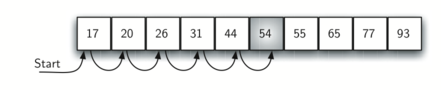
இந்த வழக்கில், வழிமுறையானது உருப்படி கண்டுபிடிக்கப்படவில்லை என்று புகாரளிக்க அனைத்து உருப்படிகளும் தொடர்ந்து பார்க்க வேண்டியதில்லை. இது உடனடியாக நிறுத்தப்படலாம். கீழேயுள்ள நிரல் தொகுப்பு தொடர்ச்சியான தேடல் செயல்பாட்டின் இந்த மாறுபாட்டைக் காட்டுகிறது.
def ordered_sequential_search(alist, item): position = 0 while position < len(alist): if alist[position] == item: return True if alist[position] > item: return False position = position + 1 return False testlist = [0, 1, 2, 8, 13, 17, 19, 32, 42,] ordered_sequential_search(testlist, 3) # => False ordered_sequential_search(testlist, 13) # => True |
கீழே உள்ள அட்டவணை இந்த முடிவுகளை சுருக்கமாகக் கூறுகிறது. சிறந்த வழக்கில் , உருப்படியை, ஒரே ஒரு உருப்படியை மட்டும் பார்த்து பட்டியலில் இல்லை என்பதை நாம் கண்டறியலாம். சராசரியாக, n/2 உருப்படிகளை மட்டுமே பார்த்த பிறகு நமக்குத் தெரியும். இருப்பினும், இந்த நுட்பம் இன்னும் O(n) ஆகும். சுருக்கமாக, நாங்கள் உருப்படியைக் கண்டுபிடிக்காத நிலையில் மட்டுமே பட்டியலை வரிசை செய்வதன் மூலம் தொடர்ச்சியான தேடல் மேம்படுத்தப்படுகிறது.
Case | Best Case | Worst Case | Average Case |
item is present | 1 | n | n/2 |
item is not present | n | n | n/2 |
7.3 இரும நிலை தேடல் - The Binary Search
எங்கள் ஒப்பீடுகளுடன் நாம் புத்திசாலித்தனமாக இருந்தால் வரிசைப்படுத்தப்பட்ட பட்டியலிலிருந்து அதிக நன்மைகளைப் பெற முடியும். தொடர்ச்சியான தேடலில், நாம் முதல் உருப்படியை ஒப்பிட்டுப் பார்க்கும்போது, முதல் உருப்படியை நாம் தேடுவது இல்லை என்றால் பார்க்க இன்னும் அதிகமான n-1 உருப்படிகள் உள்ளன. வரிசையாக பட்டியலைத் தேடுவதற்குப் பதிலாக, நடுத்தர உருப்படியை ஆராய்வதன் மூலம் இரும நிலை தேடல் தொடங்கும். அந்த உருப்படியை நாங்கள் தேடுகிறோம் என்றால், நாங்கள் முடித்துவிட்டோம். இது சரியான உருப்படி இல்லையென்றால், மீதமுள்ள உருப்படிகளில் பாதியை அகற்ற, பட்டியலின் கட்டளையிடப்பட்ட தன்மையைப் பயன்படுத்தலாம். நாம் தேடும் உருப்படி நடுத்தர உருப்படியை விட அதிகமாக இருந்தால், பட்டியலின் முழு கீழ்பகுதி மற்றும் நடுத்தர உருப்படியை மேலும் கருத்தில் கொள்வதிலிருந்து நீக்க முடியும் என்பதை நாங்கள் அறிவோம். உருப்படி, அது பட்டியலில் இருந்தால், மேல் பாதியில் இருக்க வேண்டும்.
நாம் மேல் பாதியுடன் செயல்முறையை மீண்டும் செய்யலாம். நடுத்தர உருப்படியிலிருந்து தொடங்கி நாம் தேடுவதை ஒப்பிட்டுப் பாருங்கள். மீண்டும், நாம் அதைக் கண்டுபிடிப்போம் அல்லது பட்டியலை பாதியாகப் பிரிக்கிறோம், எனவே எங்கள் சாத்தியமான தேடல் இடத்தின் மற்றொரு பெரிய பகுதியை நீக்குகிறது. கீழே உள்ள வரைபடம் இந்த வழிமுறை எவ்வாறு விரைவாக 54 என்ற மதிப்பை கண்டுபிடிக்கும் என்பதைக் காட்டுகிறது.
Binary search of an ordered list of integers
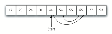
இந்த வழிமுறை ஒரு பிளவு மற்றும் வெற்றி மூலோபாயத்திற்கு ஒரு சிறந்த எடுத்துக்காட்டு ஆகும் . பிரித்து வெல்வது என்பது நாம் சிக்கலை சிறிய துண்டுகளாகப் பிரித்து, சிறிய துண்டுகளை ஏதாவது ஒரு வழியில் தீர்த்து, பின்னர் முடிவைப் பெற முழுப் பிரச்சனையையும் மீண்டும் ஒன்றிணைக்க வேண்டும். நாம் ஒரு இரும நிலைத் தேடலை பட்டியலிடும்போது, முதலில் நடுத்தர உருப்படியைச் சரிபார்க்கிறோம். நாம் தேடும் பொருள் நடுத்தர உருப்படியை விட குறைவாக இருந்தால், அசல் பட்டியலின் இடது பாதியின் இடது தேடலை நாம் செய்யலாம். அதேபோல், உருப்படி அதிகமாக இருந்தால், நாம் சரியான பாதியில் இரும நிலைத் தேடலைச் செய்யலாம். எந்த வகையிலும், இது ஒரு சிறிய பட்டியலை கடந்து செல்லும் இரும நிலைத் தேடல் செயல்பாட்டிற்கான ஒரு தொடர்ச்சியான அழைப்பு ஆகும்.
பைத்தானில் தொடர்ச்சியான இரும நிலைத் தேடலை செயல்படுத்துவது இதுபோல் தோன்றலாம்:
def binary_search(alist, item): if not alist: # list is empty -- our base case return False midpoint = len(alist) // 2 if alist[midpoint] == item: # found it! return True if item < alist[midpoint]: # item is in the first half, if at all return binary_search(alist[:midpoint], item) # otherwise item is in the second half, if at all return binary_search(alist[midpoint + 1:], item) testlist = [0, 1, 2, 8, 13, 17, 19, 32, 42] binary_search(testlist, 3) # => False binary_search(testlist, 13) # => True |
Analysis of Binary Search - இரும நிலைத்தேடல் திறணாய்வு
இரும நிலைத் தேடல் வழிமுறையை திறனாய்வு செய்ய, ஒவ்வொரு ஒப்பீடும் மீதமுள்ள உருப்படிகளில் பாதியை பரிசீலனையிலிருந்து நீக்குகிறது என்பதை நாம் நினைவில் கொள்ள வேண்டும். முழு பட்டியலையும் சரிபார்க்க இந்த வழிமுறை தேவைப்படும் அதிகபட்ச ஒப்பீடுகள் என்ன? நாம் n உருப்படிகளுடன் தொடங்கினால், முதல் ஒப்பீட்டிற்குப் பிறகு தோராயமாக n/2 உருப்படிகள் விடப்படும். இரண்டாவது ஒப்பீட்டிற்குப் பிறகு, தோராயமாக n/4 இருக்கும். பிறகு n/8, n/16, மற்றும் பல. நாம் எத்தனை முறை பட்டியலை பிரிக்கலாம்? பதிலைக் காண இந்த அட்டவணை நமக்கு உதவுகிறது:
Comparisons | Approximate Number of Items Left |
1 | n/2 |
2 | n/4 |
3 | n/8 |
... | |
i | n/2i |
நாம் பல முறை பட்டியலைப் பிரிக்கும்போது, ஒரு உருப்படியைக் கொண்ட ஒரு பட்டியலை முடிப்போம். ஒன்றில் அது நாம் தேடும் உருப்படி அல்லது அது இல்லை. எப்படியிருந்தாலும், நாங்கள் முடித்துவிட்டோம். n/2i = 1 என்று இருக்கும் போது இந்த நிலையை அடைய தேவையான ஒப்பீடுகளின் எண்ணிக்கை i ஆகும். i இற்க்கான தீர்வு எங்களுக்கு i = log[n] ஐ அளிக்கிறது. பட்டியலில் உள்ள பொருட்களின் எண்ணிக்கையைப் பொறுத்து அதிகபட்ச ஒப்பீடுகள் மடக்கை ஆகும். எனவே, இரும நிலைத் தேடல் O (log[n]) ஆகும்.
மேலே காட்டப்பட்டுள்ள தீர்வில் தொடர் அழைப்பு மூலம் ஒரு கூடுதல் திறனாய்வு சிக்கல் தீர்க்கப்பட வேண்டும்: binary_search(alist[:midpoint], item)
பட்டியலின் இடது பாதியை உருவாக்க துண்டு இயக்கியைப் (slice operator) பயன்படுத்துகிறது, அது அடுத்த அழைப்புக்கு அனுப்பப்படும் (அதேபோல் வலது பாதியிலும்). நாங்கள் மேலே செய்த பகுப்பாய்வானது துண்டு இயக்கி நிலையான நேரம் எடுக்கும் என்று கருதுகிறது. இருப்பினும், பைத்தானில் உள்ள துண்டு இயக்கி உண்மையில் O(k) என்பதை நாங்கள் அறிவோம். இதன் பொருள் துண்டு பயன்படுத்தி இரும நிலைத் தேடல் கண்டிப்பான மடக்கை நேரத்தில் செய்யாது. அதிர்ஷ்டவசமாக தொடக்க மற்றும் இறுதி குறியீடுகளுடன் பட்டியலை அனுப்புவதன் மூலம் இதை சரிசெய்ய முடியும். இந்த செயல்பாட்டை ஒரு பயிற்சியாக விட்டுவிடுகிறோம்.
தொடர்ச்சியான தேடலை விட இரும நிலைத் தேடல் பொதுவாக சிறந்தது என்றாலும், n இன் சிறிய மதிப்புகளுக்கு, வரிசைப்படுத்துவதற்கான கூடுதல் செலவு அநேகமாக மதிப்புக்குரியது அல்ல என்பதை கவனத்தில் கொள்ள வேண்டும். உண்மையில், தேடல் நன்மைகளைப் பெற வரிசைப்படுத்தும் கூடுதல் வேலையை மேற்கொள்வது செலவு குறைந்ததா என்பதை நாம் எப்போதும் கருத்தில் கொள்ள வேண்டும். நாம் ஒரு முறை வரிசைப்படுத்தி பிறகு பல முறை தேடலாம் என்றால், அந்த வகை செலவு அவ்வளவு குறிப்பிடத்தக்கதாக இருக்காது. இருப்பினும், பெரிய பட்டியல்களுக்கு, ஒரு முறை கூட வரிசைப்படுத்துவது மிகவும் விலையுயர்ந்ததாக இருக்கும், தொடக்கத்தில் இருந்து தொடர்ச்சியான தேடலைச் செய்வது சிறந்த தேர்வாக இருக்கலாம்.
7.4 Hashing - எண்ணம் அடைவாக்கம்
முந்தைய பிரிவுகளில் ஒன்றுடன் ஒன்று தொடர்புடைய உருப்படிகள் சேகரிப்பில் எங்கு சேமிக்கப்படுகின்றன என்ற தகவலைப் பயன்படுத்தி எங்கள் தேடல் வழிமுறைகளில் மேம்பாடுகளைச் செய்ய முடிந்தது. உதாரணமாக, ஒரு பட்டியல் வரிசைப்படுத்தப்பட்டுள்ளது என்பதை அறிவதன் மூலம், இருபடி(Binary) தேடலைப் பயன்படுத்தி மடக்கை நேரத்தில் தேடலாம். இந்த பிரிவில் O(1) நேரத்தில் தேடக்கூடிய தரவு கட்டமைப்பை உருவாக்குவதன் மூலம் ஒரு படி மேலே செல்ல முயற்சிப்போம். இந்த கருத்து எண்ணிம அடைவாக்கம் என்று குறிப்பிடப்படுகிறது.
இதைச் செய்வதற்கு, நாம் சேகரிப்பில் அவற்றைத் தேடப் போகும் போது உருப்படிகள் எங்கே இருக்கக்கூடும் என்பது பற்றி நாம் இன்னும் தெரிந்து கொள்ள வேண்டும். ஒவ்வொரு உருப்படியும் இருக்க வேண்டிய இடத்தில் இருந்தால், தேடலில் ஒரு உருப்படியின் இருப்பைக் கண்டறிய ஒற்றை ஒப்பீட்டைப் பயன்படுத்தலாம். எவ்வாறாயினும், இது பொதுவாக அப்படி இல்லை என்பதை நாம் பார்ப்போம்.
ஒரு எண்ணிம அடைவாக்க அட்டவணை என்பது உருப்படிகளைப் பின்னர் எளிதாகக் கண்டுபிடிக்கும் வகையில் சேமிக்கப்படும் ஒரு தொகுப்பாகும். எண்ணிம அடைவாக்க அட்டவணையின் ஒவ்வொரு நிலையும், பெரும்பாலும் பொருந்துமிடம் (slot)என்று அழைக்கப்படுகிறது அத்தோடு ஒரு உருப்படியை வைத்திருக்க முடியும் மற்றும் ஒரு முழு எண்ணின் மதிப்பில் 0. இல் இருந்து தொடங்குகிறது.உதாரணமாக, நாம் 0 என்ற பொருந்துமிடம், 1 என்ற பொருந்துமிடம், 2 என்ற பொருந்துமிடம் மற்றும் பலவற்றைக் கொண்டிருப்போம். ஆரம்பத்தில், எண்ணிம அடைவாக்க அட்டவணையில் எந்த உருப்படிகளும் இல்லை, அதனால் ஒவ்வொரு இடமும் காலியாக உள்ளது. சிறப்பு பைதான் மதிப்பு None ஆகவுள்ள ஒவ்வொரு உறுப்புடன் ஒரு பட்டியலைப் பயன்படுத்தி ஒரு எண்ணிம அடைவாக்க அட்டவணையை நாம் செயல்படுத்தலாம். கீழே உள்ள படம் m = 11 அளவு கொண்ட எண்ணிம அடைவாக்க அட்டவணையை காட்டுகிறது. வேறு வார்த்தைகளில் கூறுவதானால், 0 முதல் 10 வரை பெயரிடப்பட்ட அட்டவணையில் m இடங்கள் உள்ளன.
Hash table with 11 empty slots
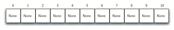
எண்ணிம அடைவாக்க அட்டவணையில் அந்த உருப்படிக்கும் பொருந்துமிடத்திற்கும் இடையிலான விவரணையாக்கம் எண்ணிம அடைவாக்க செயல்பாடு என்று அழைக்கப்படுகிறது. எண்ணிம அடைவாக்க செயல்பாடு சேகரிப்பில் உள்ள எந்த உருப்படியையும் எடுத்து, 0 மற்றும் m-1 க்கு இடையில் பொருந்துமிட பெயர்களின் வரம்பில் ஒரு முழு எண்ணை வழங்கும். நம்மிடம் முழு எண் உருப்படிகளின் தொகுப்பு 54, 26, 93, 17, 77, மற்றும் 31 உள்ளது என்று வைத்துக்கொள்வோம். சில நேரங்களில் "மீதமுள்ள முறை" என்று குறிப்பிடப்படும் எங்கள் முதல் எண்ணிம அடைவாக்க செயல்பாடு, ஒரு உருப்படியை எடுத்து அட்டவணை அளவால் பிரித்து திரும்பும் மீதமுள்ளவை அதன் எண்ணிம அடைவாக்க மதிப்பு (h (உருப்படி) = உருப்படி % 11) ஆகும் . கீழே உள்ள அட்டவணை எங்கள் எடுத்துக்காட்டு உருப்படிகளுக்கான அனைத்து எண்ணிம அடைவாக்க மதிப்புகளையும் தருகிறது. இந்த மீதமுள்ள முறை (modulo arithmetic) பொதுவாக அனைத்து எண்ணிம அடைவாக்க செயல்பாடுகளிலும் ஏதேனும் ஒரு வடிவத்தில் இருக்கும் என்பதை நினைவில் கொள்ளவும், இதன் விளைவாக பொருந்துமிட பெயர்களின் வரம்பில் இருக்க வேண்டும்.
Item | Hash Value |
54 | 10 |
26 | 4 |
93 | 5 |
17 | 6 |
77 | 0 |
31 | 9 |
எண்ணிம அடைவாக்க மதிப்புகள் கணக்கிடப்பட்டவுடன், கீழே உள்ள விளக்கத்தில் காட்டப்பட்டுள்ளபடி ஒவ்வொரு உருப்படியையும் நியமிக்கப்பட்ட நிலையில் எண்ணிம அடைவாக்க அட்டவணையில் செருகலாம். 11 இடங்களில் 6 இடங்கள் இப்போது ஆக்கிரமிக்கப்பட்டுள்ளன என்பதை நினைவில் கொள்க. இது சுமை காரணி என குறிப்பிடப்படுகிறது, இது பொதுவாக λ = numberofitems/tablesize ஆல் குறிக்கப்படுகிறது. இந்த எடுத்துக்காட்டுக்கு, λ=6/11
Hash table with six items
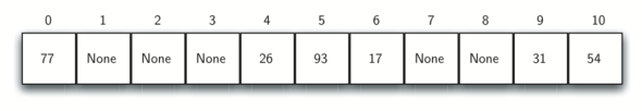
இப்போது நாம் ஒரு உருப்படியைத் தேட விரும்பும் போது, உருப்படியின் பொருந்துமிட பெயரை கணக்கிட எண்ணிம அடைவாக்க செயல்பாட்டைப் பயன்படுத்துகிறோம், பின்னர் அது இருக்கிறதா என்று எண்ணிம அடைவாக்க அட்டவணையைச் சரிபார்க்கவும். இந்த தேடுதல் செயல்பாடு O(1) ஆகும், ஏனெனில் எண்ணிம அடைவாக்க மதிப்பை கணக்கிடுவதற்கு ஒரு நிலையான நேரம் தேவைப்படுகிறது, பின்னர் அந்த இடத்தில் எண்ணிம அடைவாக்க அட்டவணையை குறியிடவும். எல்லாம் இருக்க வேண்டிய இடத்தில் இருந்தால், நாங்கள் ஒரு நிலையான நேர தேடல் வழிமுறையைக் கண்டறிந்துள்ளோம்.
ஒவ்வொரு உருப்படியும் எண்ணிம அடைவாக்க அட்டவணையில் ஒரு தனித்துவமான இடத்திற்கு விவரணையாக்கமாக இருந்தால் மட்டுமே இந்த நுட்பம் வேலை செய்யும் என்பதை நீங்கள் ஏற்கனவே பார்க்க முடியும். உதாரணமாக, எங்கள் சேகரிப்பில் அடுத்த உருப்படி 44 ஆக இருந்தால், அது 0 (44 % 11 == 0 ) என்ற எண்ணிம அடைவாக்க மதிப்பைக் கொண்டிருக்கும். 77 க்கு 0 என்ற எண்ணிம அடைவாக்க மதிப்பு இருந்ததால், எங்களுக்கு ஒரு பிரச்சனை இருக்கும். எண்ணிம அடைவாக்க செயல்பாட்டின் படி, இரண்டு அல்லது அதற்கு மேற்பட்ட உருப்படிகள் ஒரே பொருந்துமிடத்தில் இருக்க வேண்டும். இது ஒரு மோதல் (collision ) என குறிப்பிடப்படுகிறது. தெளிவாக, மோதல்கள் எண்ணிம அடைவாக்க நுட்பத்திற்கு ஒரு சிக்கலை உருவாக்குகின்றன. அவற்றைப் பற்றி பின்னர் விரிவாகப் பேசுவோம்.
Hash Functions - அடைவாக்க சார்புகள்
உருப்படிகளின் தொகுப்பைக் கொண்டு, ஒவ்வொரு உருப்படியையும் தனித்துவமான இடமாக விவரணையாக்கும் ஒரு எண்ணிம அடைவாக்க செயல்பாடு சரியான எண்ணிம அடைவாக்க செயல்பாடு என்று குறிப்பிடப்படுகிறது. உருப்படிகள் மற்றும் சேகரிப்பு ஒருபோதும் மாறாது என்று நமக்குத் தெரிந்தால், சரியான எண்ணிம அடைவாக்க செயல்பாட்டை உருவாக்க முடியும் (சரியான எண்ணிம அடைவாக்க செயல்பாடுகளைப் பற்றி மேலும் அறிய பயிற்சிகளைப் பார்க்கவும்). துரதிர்ஷ்டவசமாக, ஒரு தன்னிச்சையான உருப்படிகளின் சேகரிப்பு கொடுக்கப்பட்டால், சரியான எண்ணிம அடைவாக்க செயல்பாட்டை உருவாக்க முறையான வழி இல்லை. அதிர்ஷ்டவசமாக, செயல்திறன் ஆற்றலை பெற எண்ணிம அடைவாக்க செயல்பாடு சரியாக இருக்க வேண்டிய தேவையில்லை.
எப்போதும் சரியான எண்ணிம அடைவாக்க செயல்பாட்டைக் கொண்டிருப்பதற்கான ஒரு வழி, எண்ணிம அடைவாக்க அட்டவணையின் அளவை அதிகரிப்பதால், உருப்படி வரம்பில் சாத்தியமான ஒவ்வொரு மதிப்புக்கும் இடமளிக்க முடியும். ஒவ்வொரு உருப்படியும் ஒரு தனித்துவமான இடத்தைக் கொண்டிருக்கும் என்பதற்கு இது உத்தரவாதம் அளிக்கிறது. சிறிய எண்ணிக்கையிலான உருப்படிகளுக்கு இது நடைமுறையில் சாத்தியமானதாக இருந்தாலும், உருப்படிகளின் எண்ணிக்கை பெரியதாக இருக்கும்போது அது சாத்தியமில்லை. உதாரணமாக, உருப்படிகள் ஒன்பது இலக்க சமூக பாதுகாப்பு எண்களாக இருந்தால், இந்த முறைக்கு கிட்டத்தட்ட ஒரு பில்லியன் இடங்கள் தேவைப்படும். நாம் 25 மாணவர்களின் வகுப்பிற்கான தரவை மட்டுமே சேமிக்க விரும்பினால், நாம் மிகப்பெரிய அளவில் நினைவகத்தை வீணடிப்போம்.
மோதல்களின் எண்ணிக்கையைக் குறைக்கும், கணக்கிட எளிதானது மற்றும் எண்ணிம அடைவாக்க அட்டவணையில் உள்ள பொருட்களை சமமாக விநியோகிக்கும் ஒரு எண்ணிம அடைவாக்க செயல்பாட்டை உருவாக்குவதே எங்கள் குறிக்கோளாகும் . எளிய மீதமுள்ள முறையை நீட்டிக்க பல பொதுவான வழிகள் உள்ளன. அவற்றில் சிலவற்றை நாம் இங்கே கருத்தில் கொள்வோம்.
எண்ணிம அடைவாக்க செயல்பாடுகளை உருவாக்குவதற்கான மடிப்பு முறை (folding method) உருப்படியை சம அளவு துண்டுகளாக பிரிப்பதன் மூலம் தொடங்குகிறது (கடைசி துண்டு சம அளவு இல்லாமல் இருக்கலாம்). இதன் விளைவாக வரும் எண்ணிம அடைவாக்க மதிப்பை வழங்க இந்த துண்டுகள் ஒன்றாக சேர்க்கப்படுகின்றன. உதாரணமாக, எங்கள் உருப்படி தொலைபேசி எண் 436-555-4601 என்றால், நாங்கள் இலக்கங்களை எடுத்து 2 குழுக்களாகப் (43,65,55,46,01) பிரிப்போம். 43+65+55+46+01 ஐ சேர்த்த பிறகு, நமக்கு 210 கிடைக்கும். எங்கள் எண்ணிம அடைவாக்க அட்டவணையில் 11 இடங்கள் இருப்பதாகக் கருதினால், 11 ஐப் பிரித்து எஞ்சியதை வைத்து கூடுதல் படி செய்ய வேண்டும். 210 % 11 என்ற இந்த வழக்கில் விடை 1 ஆகும், எனவே தொலைபேசி எண் 436-555-4601 ஆனது பொருந்துமிடம் 1 இற்கு எண்ணிம அடைவாக்கம் செய்யப்படும். சில மடிப்பு முறைகள் ஒரு படி மேலே சென்று சேர்ப்பதற்கு முன் மற்ற ஒவ்வொரு பகுதியையும் தலைகீழாக மாற்றும். மேலே உள்ள எடுத்துக்காட்டுக்கு, நாங்கள் 43+56+55+64+01 = 219 பெறுகிறோம் 219 % 11 = 10 ஆகும்.
எண்ணிம அடைவாக்க செயல்பாட்டை உருவாக்குவதற்கான மற்றொரு எண் நுட்பம் mid-square method என்று அழைக்கப்படுகிறது. நாங்கள் முதலில் உருப்படியை சதுரமாக்கி, அதன் விளைவாக வரும் இலக்கங்களின் சில பகுதியை பிரித்தெடுக்கிறோம். உதாரணமாக, உருப்படி 44 ஆக இருந்தால், நாங்கள் முதலில் 442 = 1,936ஐ கணக்கிடுவோம். நடுவிலுள்ள இரண்டு இலக்கங்களை பிரித்தெடுப்பதன் மூலம் 93 ஐயும் , மற்றும் மீதமுள்ள படிநிலையை செயல்படுத்துவதன் மூலம், நாம் 5 (93 % 11) பெறுகிறோம். கீழே உள்ள அட்டவணை மீதமுள்ள முறை மற்றும் mid-square method இரண்டின் கீழ் உள்ள உருப்படிகளைக் காட்டுகிறது. இந்த மதிப்புகள் எவ்வாறு கணக்கிடப்பட்டன என்பதை நீங்கள் புரிந்துகொண்டீர்கள் என்பதை நீங்கள் சரிபார்க்க வேண்டும்.
Item | Remainder | Mid-Square |
54 | 10 | 3 |
26 | 4 | 7 |
93 | 5 | 9 |
17 | 6 | 8 |
77 | 0 | 4 |
31 | 9 | 6 |
சரங்கள் போன்ற எழுத்து அடிப்படையிலான பொருட்களுக்கான எண்ணிம அடைவாக்க செயல்பாடுகளையும் நாம் உருவாக்கலாம். "Cat" என்ற வார்த்தையை சாதாரண மதிப்புகளின் வரிசையாகக் கருதலாம்.
>>> ord('c') 99 >>> ord('a') 97 >>> ord('t') 116 |
இந்த மூன்று சாதாரண மதிப்புகளை எடுத்து, அவற்றைச் சேர்த்து, மீதமுள்ள முறையைப் பயன்படுத்தி எண்ணிம அடைவாக்க மதிப்பைப் பெறலாம்.
Hashing a string using ordinal values
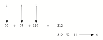
hash எனப்படும் ஒரு செயல்பாடு கீழே உள்ளது, அது ஒரு சரம் மற்றும் அட்டவணை அளவை எடுத்து, எண்ணிம அடைவாக்க மதிப்பை 0 முதல் tablesize - 1 வரை அளிக்கிறது.
def hash(astring, tablesize): the_sum = sum(ord(char) for char in astring) return the_sum % tablesize |
இந்த எண்ணிம அடைவாக்க செயல்பாட்டைப் பயன்படுத்தும் போது, ஓரெழுத்து இருசொற்களுக்கு (anagrams) எப்போதும் ஒரே எண்ணிம அடைவாக்க மதிப்பு வழங்கப்படும் என்பது குறிப்பிடத்தக்கது. இதைச் சரிசெய்ய, குறியுருவின் நிலையை நாம் ஒரு எடையாகப் பயன்படுத்தலாம். கீழேயுள்ள விளக்கமானது, நிலை மதிப்பை ஒரு எடை காரணியாகப் பயன்படுத்துவதற்கான ஒரு சாத்தியமான வழியைக் காட்டுகிறது. hash செயல்பாட்டில் மாற்றம் ஒரு பயிற்சியாக விடப்படுகிறது.
Hashing a String Using Ordinal Values with Weighting
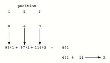
ஒரு தொகுப்பில் உள்ள உருப்படிகளுக்கான எண்ணிம அடைவாக்க மதிப்புகளைக் கணக்கிடுவதற்கான பல கூடுதல் வழிகளை நீங்கள் சிந்திக்கலாம். நினைவில் கொள்ள வேண்டிய முக்கியமான விஷயம் என்னவென்றால், எண்ணிம அடைவாக்க செயல்பாடு திறமையாக இருக்க வேண்டும், அதனால் அது சேமிப்பு மற்றும் தேடல் செயல்முறையின் மேலாதிக்க பகுதியாக மாறாது. எண்ணிம அடைவாக்க செயல்பாடு மிகவும் சிக்கலானதாக இருந்தால், முன்பு விவரிக்கப்பட்டபடி ஒரு அடிப்படை தொடர்ச்சியான அல்லது இரும நிலைத் தேடலைச் செய்வதை விட பொருந்துமிட பெயரை கணக்கிடுவது அதிக வேலை ஆகிறது. இது எண்ணிம அடைவாக்கத்தின் நோக்கத்தை விரைவாக தோற்கடிக்கும்.
Collision Resolution - அடைவாக்கத்தில் தனித்துவம் காத்தல்
நாங்கள் இப்போது மோதல்களின் பிரச்சனைக்குத் திரும்புகிறோம். இரண்டு உருப்படிகள் ஒரே இடத்திற்கு எண்ணிம அடைவாக்கம் செய்யும்போது, இரண்டாவது உருப்படியை எண்ணிம அடைவாக்க அட்டவணையில் வைப்பதற்கான முறையான முறையை நாம் கொண்டிருக்க வேண்டும். இந்த செயல்முறை மோதல் தீர்மானம் என்று அழைக்கப்படுகிறது. நாம் முன்பு கூறியது போல், எண்ணிம அடைவாக்க செயல்பாடு சரியாக இருந்தால், மோதல்கள் ஏற்படாது. இருப்பினும், இது பெரும்பாலும் சாத்தியமில்லை என்பதால், மோதல் தீர்மானம் எண்ணிம அடைவாக்கத்தில் மிக முக்கியமான பகுதியாகிறது.
மோதல்களைத் தீர்ப்பதற்கான ஒரு முறை எண்ணிம அடைவாக்க அட்டவணையைப் பார்த்து மோதலுக்கு காரணமான உருப்படியைப் பிடிக்க மற்றொரு திறந்த இடத்தைக் கண்டுபிடிக்க முயற்சிக்கிறது. இதைச் செய்வதற்கான ஒரு எளிய வழி, அசல் எண்ணிம அடைவாக்க மதிப்பு நிலையில் தொடங்கி பின்னர் காலியாக இருக்கும் முதல் பொருந்துமிடத்தை நாம் சந்திக்கும் வரை இடங்கள் வழியாக தொடர்ச்சியான முறையில் நகர்வது ஆகும் . முழு எண்ணிம அடைவாக்க அட்டவணையை மறைப்பதற்கு நாம் முதல் இடத்திற்கு (வட்டமாக) திரும்ப வேண்டியிருக்கலாம் என்பதை நினைவில் கொள்க. இந்த மோதல் தீர்மான செயல்முறை திறந்த முகவரியாக்கம் (open addressing ) என குறிப்பிடப்படுகிறது, அதில் எண்ணிம அடைவாக்க அட்டவணையில் அடுத்த திறந்த பொருந்துமிடம் அல்லது முகவரியைக் கண்டுபிடிக்க முயற்சிக்கிறது. ஒவ்வொரு இடத்தையும் முறையாகப் பார்வையிடுவதன் மூலம், நேரியல் ஆய்வு (linear probing) எனப்படும் திறந்த முகவரி நுட்பத்தை நாங்கள் செய்கிறோம்.
கீழேயுள்ள விளக்கமானது எளிய மீதமுள்ள முறை எண்ணிம அடைவாக்க செயல்பாட்டின் கீழ் முழு எண் உருப்படிகளின் விரிவாக்கப்பட்ட தொகுப்பைக் காட்டுகிறது(54, 26, 93, 17, 77, 31, 44, 55, 20). 44 ஐ பொருந்துமிடம் 0 இல் வைக்க முயற்சிக்கும்போது, ஒரு மோதல் ஏற்படுகிறது. நேரியல் ஆய்வின் கீழ், நாம் ஒரு திறந்த நிலையை கண்டுபிடிக்கும் வரை, தொடர்ச்சியாக, பொருந்துமிடத்தைப் பார்க்கிறோம். இந்த வழக்கில், பொருந்துமிடம் 1 ஐக் காணலாம்.
மீண்டும், 55 ஆனது பொருந்துமிடம் 0 இல் செல்ல வேண்டும் ஆனால் அது அடுத்த திறந்த நிலை என்பதால் பொருந்துமிடம் 2 இல் வைக்கப்பட வேண்டும். 20 எண்ணிம அடைவாக்கத்தின் இறுதி மதிப்பு பொருந்துமிடம் 9 இற்காகும் . பொருந்துமிடம் 9 நிரம்பியிருப்பதால், நாம் நேரியல் ஆய்வு செய்யத் தொடங்குகிறோம். நாங்கள் 10, 0, 1 மற்றும் 2 இடங்களைப் பார்வையிடுகிறோம், இறுதியாக 3 வது இடத்தில் ஒரு வெற்று இடத்தைக் கண்டுபிடிப்போம்.
Collision resolution with linear probing
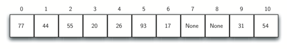
திறந்த முகவரி மற்றும் நேரியல் ஆய்வைப் பயன்படுத்தி நாங்கள் ஒரு எண்ணிம அடைவாக்க அட்டவணையை உருவாக்கியவுடன், உருப்படிகளைத் தேட அதே முறைகளைப் பயன்படுத்துவது அவசியம். நாம் உருப்படியைப் பார்க்க விரும்புகிறோம் என்று வைத்துக்கொள்வோம். எண்ணிம அடைவாக்க மதிப்பை கணக்கிடும்போது, நமக்கு 5 கிடைக்கும். பொருந்துமிடம் 5 இல் பார்த்தால் 93 இருப்பது தெரியவருகிறது, மேலும் நாம் True ஐ திரும்ப பெறலாம். நாம் 20 ஐ தேடுகிறோம் என்றால் என்ன செய்வது? இப்போது எண்ணிம அடைவாக்க மதிப்பு 9, மற்றும் பொருந்துமிடம் 9 தற்போது 31 ஐ வைத்திருக்கிறது. மோதல்கள் இருக்கக்கூடும் என்று எங்களுக்குத் தெரிந்ததால், False ஐ நாங்கள் திருப்பித் தர முடியாது. நாம் இப்போது தொடர்ச்சியான தேடலை செய்ய வேண்டிய கட்டாயத்தில் இருக்கிறோம், நிலை 10 ல் தொடங்கி, ஒன்று உருப்படியை கண்டுபிடிக்கும் வரை அல்லது ஒரு வெற்று இடத்தைக் கண்டுபிடிக்கும் வரை பார்க்கிறோம்.
நேரியல் ஆய்வுக்கு ஒரு குறைபாடு கொத்தாக்கம் (clustering) ஆகும் ; உருப்படிகள் அட்டவணையில் கொத்தாக இருக்கும். இதன் பொருள் ஒரே எண்ணிம அடைவாக்க மதிப்பில் பல மோதல்கள் ஏற்பட்டால், சுற்றியுள்ள பல இடங்கள் நேரியல் ஆய்வு தீர்மானத்தால் நிரப்பப்படும். மேலே உள்ள 20 ஐ சேர்க்க நாங்கள் முயன்றபோது பார்த்தபடி, செருகப்படும் மற்ற பொருட்களின் மீது இது தாக்கத்தை ஏற்படுத்தும். இறுதியாக ஒரு திறந்த நிலையைக் கண்டுபிடிக்க மதிப்புகளின் கொத்தாக்கம் 0 க்குத் தவிர்க்கப்பட வேண்டும். இந்த கொத்தாக்கம் கீழே காட்டப்பட்டுள்ளது.
A cluster of items for slot 0
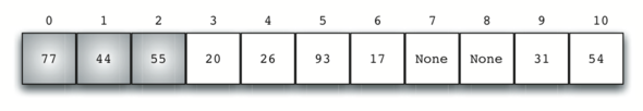
கொத்தாக்கத்தை கையாள்வதற்கான ஒரு வழி, நேரியல் ஆய்வு நுட்பத்தை விரிவாக்குவது ஆகும், இதனால் அடுத்த திறந்த இடத்திற்கு தொடர்ச்சியாகப் பார்ப்பதற்குப் பதிலாக, நாங்கள் இடங்களைத் தவிர்த்து, மோதல்களை ஏற்படுத்திய பொருட்களை இன்னும் சமமாக விநியோகிக்கிறோம். இது சாத்தியமான கொத்தாக்கத்தைக் குறைக்கும். கீழே உள்ள விளக்கப்படம் “plus 3” ஆய்வு மூலம் மோதல் தீர்மானம் செய்யப்படும்போது உருப்படிகளைக் காட்டுகிறது. இதன் பொருள், ஒரு முறை மோதல் ஏற்பட்டால், காலியாக இருக்கும் ஒன்றைக் கண்டுபிடிக்கும் வரை ஒவ்வொரு மூன்றாவது இடத்தையும் பார்ப்போம்.
Collision resolution using “plus 3”
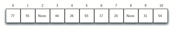
மோதலுக்குப் பிறகு மற்றொரு இடத்தைத் தேடும் இந்த செயல்முறையின் பொதுவான பெயர் மறு எண்ணிம அடைவாக்கமாகும்(rehashing). எளிமையான நேரியல் ஆய்வுடன், மறு எண்ணிம அடைவாக்கமாகும் செயல்பாடு என்பது newhashvalue = rehash(oldhashvalue), அங்கு rehash(pos) = (pos + 1) % sizeoftable ஆகும் . "plus 3" மறு எண்ணிம அடைவாக்கத்தை (pos) = (pos+3) % sizeoftable என வரையறுக்கலாம். பொதுவாக,rehash(pos) = (pos + skip) % sizeoftable ஆகும் . "skip" அளவு அட்டவணையில் உள்ள அனைத்து இடங்களும் இறுதியில் பார்வையிடப்படும் வகையில் இருக்க வேண்டும் என்பதை கவனத்தில் கொள்ள வேண்டும். இல்லையெனில், அட்டவணையின் ஒரு பகுதி பயன்படுத்தப்படாது. இதை உறுதி செய்ய, அட்டவணை அளவு ஒரு முதன்மை எண் என்று அடிக்கடி பரிந்துரைக்கப்படுகிறது. எங்கள் உதாரணங்களில் நாங்கள் 11 ஐப் பயன்படுத்துவதற்கான காரணம் இதுதான்.
நேரியல் ஆய்வு யோசனையின் மாறுபாடு இருபடி ஆய்வு (quadratic probing) என்று அழைக்கப்படுகிறது. நிலையான "skip" மதிப்பைப் பயன்படுத்துவதற்குப் பதிலாக, எண்ணிம அடைவாக்க மதிப்பை 1, 3, 5, 7, 9 மற்றும் பலவற்றால் அதிகரிக்கும் மறு எண்ணிம அடைவாக்கும் செயல்பாட்டைப் பயன்படுத்துகிறோம். இதன் பொருள் முதல் எண்ணிம அடைவாக்க மதிப்பு h என்றால், அடுத்தடுத்த மதிப்புகள் h+1, h+4, h+9, h+16, மற்றும் பல. வேறு வார்த்தைகளில் கூறுவதானால், இருபடி ஆய்வு தொடர்ச்சியான சரியான சதுரங்களைக் கொண்ட ஒரு skip ஐ பயன்படுத்துகிறது. கீழேயுள்ள விளக்கப்படம் இந்த நுட்பத்தைப் பயன்படுத்தி வைக்கப்பட்ட பிறகு எங்கள் எடுத்துக்காட்டு மதிப்புகளைக் காட்டுகிறது.
Collision resolution with quadratic probing
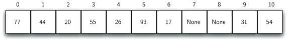
மோதல் பிரச்சனையை கையாள்வதற்கான ஒரு மாற்று முறை, ஒவ்வொரு பொருந்துமிடத்திற்கும் ஒரு தொகுப்பு (அல்லது சங்கிலி) உருப்படிகளின் குறிப்பை வைத்திருக்க அனுமதிப்பது. சங்கிலிப் பிணைப்பு (Chaining ) எண்ணிம அடைவாக்க அட்டவணையில் ஒரே இடத்தில் பல உருப்படிகளை இருக்க அனுமதிக்கிறது. மோதல்கள் நிகழும்போது, உருப்படி இன்னும் எண்ணிம அடைவாக்க அட்டவணையின் சரியான பொருந்துமிடத்தில் வைக்கப்படுகிறது. ஒரே இடத்திற்கு அதிகமான உருப்படிகள் எண்ணிம அடைவாக்கம் செய்யப்படுவதால், சேகரிப்பில் உள்ள உருப்படிகளைத் தேடுவதில் சிரமம் அதிகரிக்கிறது. கீழே உள்ள விளக்கம் உருப்படிகளைக் காட்டுகிறது, அவை மோதல்களைத் தீர்க்க சங்கிலியைப் பயன்படுத்தும் எண்ணிம அடைவாக்க அட்டவணையில் சேர்க்கப்படுகின்றன.
Collision resolution with chaining
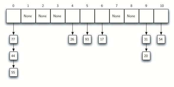
நாம் ஒரு உருப்படியைத் தேட விரும்பும் போது, எண்ணிம அடைவைக்க செயல்பாட்டைப் பயன்படுத்தி அது வசிக்க வேண்டிய இடத்தை உருவாக்குகிறது. ஒவ்வொரு பொருந்துமிடத்திற்கும் ஒரு தொகுப்பைக் கொண்டிருப்பதால், உருப்படி இருக்கிறதா என்பதைத் தேடுவதற்கு ஒரு தேடல் நுட்பத்தைப் பயன்படுத்துகிறோம். நன்மை என்னவென்றால், சராசரியாக ஒவ்வொரு பொருந்துமிடத்திலும் பல குறைவான உருப்படிகள் இருக்கலாம், எனவே தேடல் ஒருவேளை மிகவும் திறமையானதாக இருக்கும்.
Analysis of Hashing - அடைவாக்கம் திறணாய்வு
சிறந்த வழக்கில் எண்ணிம அடைவு ஒரு O (1) மற்றும் நிலையான நேர தேடல் நுட்பத்தை வழங்கும் என்று நாங்கள் முன்பு கூறினோம். இருப்பினும், மோதல்கள் காரணமாக, ஒப்பீடுகளின் எண்ணிக்கை பொதுவாக அவ்வளவு எளிதல்ல. எண்ணிம அடைவின் முழுமையான திறனாய்வு இந்த உரையின் எல்லைக்கு அப்பாற்பட்டதாக இருந்தாலும், ஒரு உருப்படியைத் தேடுவதற்குத் தேவையான ஒப்பீடுகளின் எண்ணிக்கையை தோராயமாக அளிக்கும் சில நன்கு அறியப்பட்ட முடிவுகளை நாம் கூறலாம்.
ஒரு எண்ணிம அடைவாக்க அட்டவணையின் பயன்பாட்டை நாம் திறனாய்வு செய்ய வேண்டிய மிக முக்கியமான தகவல் சுமை காரணி, λ ஆகும் . கருத்தியல் ரீதியாக, λ சிறியதாக இருந்தால், மோதல்கள் ஏற்படுவதற்கான வாய்ப்புகள் குறைவு, அதாவது உருப்படிகள் அவர்கள் இருக்கும் இடங்களில் அதிகமாக இருக்கும். λ பெரியதாக இருந்தால், அட்டவணை நிரம்புகிறது என்று அர்த்தம், மேலும் மேலும் மோதல்கள் உள்ளன. இதன் பொருள் மோதல் தீர்மானம் மிகவும் கடினம், வெற்று பொருந்துமிடத்தை கண்டுபிடிக்க அதிக ஒப்பீடுகள் தேவை. சங்கிலியால், அதிகரித்த மோதல்கள் என்பது ஒவ்வொரு சங்கிலியிலும் அதிக எண்ணிக்கையிலான உருப்படிகளின் எண்ணிக்கையைக் குறிக்கிறது.
முன்பு போலவே, வெற்றிகரமான மற்றும் தோல்வியுற்ற தேடலுக்கான முடிவை நாங்கள் பெறுவோம். நேரியல் ஆய்வுகளுடன் திறந்த முகவரியைப் பயன்படுத்தி வெற்றிகரமான தேடலுக்கு, சராசரி ஒப்பீடுகளின் எண்ணிக்கை தோராயமாக ½(1+1/[1−λ]) ஆகும். மற்றும் தோல்வியுற்ற தேடல் ½(1+1/[1-λ]2) அளிக்கிறது நாம் சங்கிலியைப் பயன்படுத்துகிறோம் என்றால், ஒப்பீடுகளின் சராசரி எண்ணிக்கை வெற்றிகரமான வழக்கிற்கு 1 + λ/2 ஆகும் , தேடல் தோல்வியுற்றால் ஒப்பீடுகள் λ ஆகும்.
8. Trees - இருகிளை மரம் தரவமைப்பு
8.1 Introduction to Trees - இருகிளை மரம் தரவமைப்பு அறிமுகம்
மர தரவுவகை என்பது பொதுவாக எதிர்கொள்ளும் தரவு வடிவமாகும், இது படிநிலை தொடர்புகளை பிரதிநிதித்துவப்படுத்த அனுமதிக்கிறது.
மென்பொருளை எழுதும் போது நாம் சந்திக்கும் பல படிநிலையானது கட்டமைப்புகளைச் செய்ய வேண்டும். உதாரணமாக, ஒரு கோப்பு முறைமையில் உள்ள ஒவ்வொரு கோப்பும் கோப்பகமும் வேர் கோப்பகம் வரை ஒரே ஒரு பெற்றோர் கோப்பகத்தின் “inside” இருக்கும். ஒரு HTML ஆவணத்தில், ஒவ்வொரு குறிச்சொல்லும் root (html) குறிச்சொல் வரை ஒரே ஒரு பெற்றோர் குறிச்சொல்லின் உள்ளே இருக்கும்.
முனை ஓரம் அடைவு போன்ற பயனுள்ள தரவு கட்டமைப்புகளைச் செயல்படுத்தவும், விரைவான தேடல்களைச் செய்யவும் மாற தரவுவகைகளைப் பயன்படுத்தலாம் என்பதும் மாறிவிடும். இந்த பிரிவில் மாற தரவு வகைகளுக்கான பல பயன்பாட்டு நிகழ்வுகளில் சிலவற்றையும், மாற தரவுவகைகள் வழியாக பயணிப்பதற்கான வழிமுறைகளை ஆராய்வோம்.
Examples of trees - இருகிளை மரம் உதாரணங்கள்
மர தரவு கட்டமைப்புகள் அவற்றின் தாவரவியல் உறவினர்களுடன் பொதுவான பல விஷயங்களைக் கொண்டுள்ளன. இரண்டிற்கும் வேர், கிளைகள் மற்றும் இலைகள் உள்ளன. ஒரு வித்தியாசம் என்னவென்றால், ஒரு மர தரவு கட்டமைப்பின் வேர் "மேல்" இருக்க வேண்டும் என்று கருதுவது மிகவும் உள்ளுணர்வாக உள்ளது, உதாரணமாக ஒரு கோப்பு முறைமையின் வேர் அதன் துணை அடைவுகளுக்கு "மேலே" உள்ளது.
மர தரவு கட்டமைப்புகள் பற்றிய எங்கள் ஆய்வைத் தொடங்குவதற்கு முன், சில பொதுவான எடுத்துக்காட்டுகளைப் பார்ப்போம்
ஒரு மரத்தின் முதல் உதாரணம் உயிரியலில் இருந்து ஒரு வகைப்பாடு மரம். கீழே உள்ள விளக்கம் சில விலங்குகளின் உயிரியல் வகைப்பாட்டின் உதாரணத்தைக் காட்டுகிறது. இந்த எளிய உதாரணத்திலிருந்து, மரங்களின் பல பண்புகளைப் பற்றி அறிந்து கொள்ளலாம். இந்த உதாரணம் நிரூபிக்கும் முதல் பண்பு மரங்கள் படிநிலையானது. படிநிலை மூலம், மரங்கள் அடுக்குகளில் கட்டமைக்கப்பட்டுள்ளன என்று அர்த்தம், மேலே உள்ள பொதுவான விஷயங்கள் மற்றும் கீழே உள்ள மிகவும் குறிப்பிட்ட விஷயங்கள். படிநிலையின் மேல் பகுதி இராச்சியம், மரத்தின் அடுத்த அடுக்கு (மேலே உள்ள அடுக்கின் "குழந்தைகள்") ஃபைலம், பின்னர் வகுப்பு மற்றும் பல. இருப்பினும், வகைப்பாடு மரத்தில் நாம் எவ்வளவு ஆழமாகச் சென்றாலும், அனைத்து உயிரினங்களும் இன்னும் விலங்குகளாகவே இருக்கின்றன.
Taxonomy of some common animals shown as a tree

நீங்கள் மரத்தின் உச்சியில் இருந்து தொடங்கி கீழே வரை வட்டங்கள் மற்றும் அம்புகளால் ஆன பாதையைப் பின்பற்றலாம் என்பதைக் கவனியுங்கள். மரத்தின் ஒவ்வொரு நிலையிலும் நாம், நம்மை நாமே ஒரு கேள்வியைக் கேட்டுக்கொள்ளலாம், அதன் பிறகு நமது பதிலுக்கு உடன்படும் பாதையைப் பின்பற்றலாம். உதாரணமாக, "இந்த விலங்கு ஒரு Chordate அல்லது Arthropod?" என்று நாம் கேட்கலாம். பதில் Chordate என்றால், அந்த வழியைப் பின்பற்றி, “இது ஒரு பாலூட்டியா?” என்று கேட்கிறோம். இல்லையென்றால், நாங்கள் சிக்கிக் கொள்கிறோம் (ஆனால் இந்த எளிமைப்படுத்தப்பட்ட எடுத்துக்காட்டில் மட்டுமே). நாம் பாலூட்டி மட்டத்தில் இருக்கும்போது, "இந்த பாலூட்டி ஒரு விலங்கினமா அல்லது மாமிச உண்ணியா?" நாம் பொதுவான பெயரைக் கொண்ட மரத்தின் அடிப்பகுதிக்குச் செல்லும் வரை பாதைகளைப் பின்பற்றலாம்.
.
நீங்கள் மரத்தின் உச்சியில் இருந்து தொடங்கி கீழே வரை வட்டங்கள் மற்றும் அம்புகளால் ஆன பாதையைப் பின்பற்றலாம் என்பதைக் கவனியுங்கள். மரத்தின் ஒவ்வொரு நிலையிலும் நாம், நம்மை நாமே ஒரு கேள்வியைக் கேட்டுக்கொள்ளலாம், அதன் பிறகு நமது பதிலுக்கு உடன்படும் பாதையைப் பின்பற்றலாம். உதாரணமாக, "இந்த விலங்கு ஒரு Chordate அல்லது Arthropod?" என்று நாம் கேட்கலாம். பதில் Chordate என்றால், அந்த வழியைப் பின்பற்றி, “இது ஒரு பாலூட்டியா?” என்று கேட்கிறோம். இல்லையென்றால், நாங்கள் சிக்கிக் கொள்கிறோம் (ஆனால் இந்த எளிமைப்படுத்தப்பட்ட எடுத்துக்காட்டில் மட்டுமே). நாம் பாலூட்டி மட்டத்தில் இருக்கும்போது, "இந்த பாலூட்டி ஒரு விலங்கினமா அல்லது மாமிச உண்ணியா?" நாம் பொதுவான பெயரைக் கொண்ட மரத்தின் அடிப்பகுதிக்குச் செல்லும் வரை பாதைகளைப் பின்பற்றலாம்.
மரங்களின் இரண்டாவது சொத்து என்னவென்றால், ஒரு முனையின் அனைத்து குழந்தைகளும் மற்றொரு முனையின் குழந்தைகளிலிருந்து சுயாதீனமாக உள்ளன. உதாரணமாக, Felis இனத்திற்கு Domestica மற்றும் Leo என்ற குழந்தைகள் உள்ளனர். Musca இனத்திற்கும் Domestica என்ற குழந்தை உள்ளது, ஆனால் அது வேறுபட்ட முனை மற்றும் Felis இன் Domestica குழந்தையிலிருந்து சுயாதீனமானது. அதாவது, Felis இன் குழந்தையை பாதிக்காமல், Musca இன் குழந்தையாக இருக்கும் முனையை மாற்றலாம்.
மூன்றாவது பண்பு என்னவென்றால், ஒவ்வொரு இலை முனையும் தனித்துவமானது. விலங்கு இராச்சியத்தில் உள்ள ஒவ்வொரு இனத்தையும் தனித்துவமாக அடையாளம் காணும் மரத்தின் வேரிலிருந்து இலை வரையிலான பாதையை நாம் குறிப்பிடலாம்; எடுத்துக்காட்டாக, Animalia → Chordate \rightarrow Mammal → Carnivora → Felidae → Felis → Domestica.
நீங்கள் ஒவ்வொரு நாளும் பயன்படுத்தும் மர அமைப்புக்கான மற்றொரு உதாரணம் ஒரு கோப்பு முறைமை. ஒரு கோப்பு அமைப்பில், கோப்பகங்கள் அல்லது கோப்புறைகள் ஒரு மரமாக கட்டமைக்கப்படுகின்றன
A small part of the unix file system hierarchy
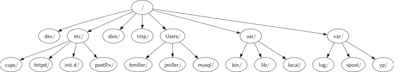
கோப்பு முறைமை மரமானது உயிரியல் வகைப்பாடு மரத்துடன் மிகவும் பொதுவானது. நீங்கள் வேரிலிருந்து எந்த கோப்பகத்திற்கும் ஒரு பாதையை பின்பற்றலாம். அந்த பாதை அந்த துணை அடைவு (மற்றும் அதில் உள்ள அனைத்து கோப்புகளையும்) தனித்துவமாக அடையாளம் காட்டும். மரங்களின் மற்றொரு முக்கியமான சொத்து, அவற்றின் படிநிலை இயல்பிலிருந்து பெறப்பட்டது, நீங்கள் ஒரு மரத்தின் முழுப் பகுதிகளையும் (துணை மரம் என்று அழைக்கப்படுகிறது) மரத்தின் கீழ் நிலைகளை பாதிக்காமல் வேறு இடத்திற்கு நகர்த்தலாம். எடுத்துக்காட்டாக, /etc/ இல் தொடங்கும் முழு துணை மரத்தையும் எடுத்து, வேரிலிருந்து பிரித்தெடுக்கலாம் மற்றும் usr/ கீழ் மீண்டும் இணைக்கலாம். இது தனிப்பட்ட பாதைப்பெயரை httpd என /etc/httpd இலிருந்து /usr/etc/httpd என மாற்றும், ஆனால் httpd கோப்பகத்தின் உள்ளடக்கங்கள் அல்லது குழந்தைகளை பாதிக்காது.
ஒரு மரத்தின் இறுதி உதாரணம் ஒரு வலைப்பக்கம். HTML ஐப் பயன்படுத்தி எழுதப்பட்ட எளிய வலைப்பக்கத்தின் உதாரணம் கீழே உள்ளது.
<html>
<head>
<title>simple</title>
</head>
<body>
<h1>A simple web page</h1>
<ul>
<li>List item one</li>
<li>List item two</li>
</ul>
<h2><a href="https://www.google.com">Google</a><h2>
</body>
</html>
வலைப்பக்கத்தை உருவாக்கப் பயன்படுத்தப்படும் HTML குறிச்சொற்கள் ஒவ்வொன்றிற்கும் பொருந்தக்கூடிய மரம் இங்கே உள்ளது.
A tree corresponding to the markup elements of a web page
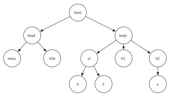
HTML மூலக் குறியீடு மற்றும் மூலத்துடன் இணைந்த மரம் மற்றொரு படிநிலையை விளக்குகின்றன. மரத்தின் ஒவ்வொரு நிலையும் HTML குறிச்சொற்களுக்குள் உள்ளாக அமைக்கப்படும் நிலைக்கு ஒத்திருப்பதைக் கவனியுங்கள். மூலத்தில் உள்ள முதல் குறிச்சொல் மற்றும் கடைசி . பக்கத்தில் உள்ள அனைத்து குறிச்சொற்களும் ஜோடிக்குள் உள்ளன. நீங்கள் சரிபார்த்தால், இந்த உள்ளாக அமைக்கப்படும் பண்பு மரத்தின் அனைத்து மட்டங்களிலும் உண்மையாக இருப்பதை நீங்கள் காண்பீர்கள்.
வரையறைகள் (Definitions)
இப்போது நாம் மரங்களின் உதாரணங்களைப் பார்த்தோம், நாம் மரம் மற்றும் அதன் கூறுகளை முறையாக வரையறுப்போம்.
உச்சி ( Node )
ஒரு உச்சி என்பது ஒரு மரத்தின் அடிப்படை பகுதியாகும். இது ஒரு தனித்துவமான பெயரைக் கொண்டிருக்கலாம் சில நேரங்களில் "சாவி " என்று அழைக்கவும். ஒரு முனையில் கூடுதலான தகவல்களும் இருக்கலாம் இந்த புத்தகத்தில் “payload.” என்று குறிப்பிடப்படுகின்றது. “payload.” தகவல்கள் பல மர தரவமைப்பு வழிமுறைகளுக்கு மையமானது அல்ல.மாற தரவமைப்புக்களைப் பயன்படுத்தும் பயன்பாடுகளில் பெரும்பாலும் முக்கியமானதாகும்.
விளிம்பு (Edge)
ஒரு விளிம்பு ஒரு மரத்தின் மற்றொரு அடிப்படை பகுதியாகும். ஒரு விளிம்பு இரண்டு உச்சிகளை இணைக்கிறது அவர்களுக்கு இடையே ஒரு தொடர்பு இருப்பதைக் காட்டுகிறது. வேர் தவிர மற்ற ஒவ்வொரு கணு மற்றொரு உச்சியிலிருந்து சரியாக ஒரு உள்வரும் விளிம்பில் இணைக்கப்பட்டுள்ளது. ஒவ்வொரு உச்சியிலும் பல வெளிச்செல்லும் விளிம்புகள் இருக்கலாம்.
வேர் (Root)
மரத்தின் வேர் மட்டுமே மரத்தில் உள்வரும் விளிம்புகள் இல்லாத ஒரே உச்சியாகும் .ஒரு கோப்பு முறைமையில் , / என்பது மரத்தின் வேர். HTML ஆவணத்தில், <html> tag என்பது மரத்தின் வேர்.
பாதை (Path)
பாதை என்பது விளிம்புகளால் இணைக்கப்பட்ட உச்சிகளின் வரிசைப்படுத்தப்பட்ட பட்டியலாகும். எடுத்துக்காட்டாக, பாலூட்டி → Carnivora → Felidae → Felis → Domestica என்பது ஒரு பாதை.
குழந்தைகள் (Children)
ஒரே முனையிலிருந்து உள்வரும் விளிம்புகளைக் கொண்ட c முனைகளின் தொகுப்பு அந்த முனையின் குழந்தைகளாக இருக்க வேண்டும். எங்கள் கோப்பு முறைமை எடுத்துக்காட்டில், உச்சிகள் log/, spool/,மற்றும் yp/ ஆகியவை உச்சி var/ இன் குழந்தைகள் ஆகும்.
பெற்றோர் (Parent)
வெளிச்செல்லும் விளிம்புகளுடன் இணைக்கும் உச்சி பெற்றோர் ஆகும்.எங்கள் கோப்பு முறைமை எடுத்துக்காட்டில், உச்சி var/ என்பது உச்சிகள் log/, spool/,மற்றும் yp/ இன் பெற்றோர் ஆகும்.
உடன்பிறப்புகள் (Sibling)
ஒரே பெற்றோரின் குழந்தைகளான மரத்தில் உள்ள கணுக்கள் உடன்பிறப்புகள் என்று கூறப்படுகிறது. உச்சிகால etc/ மற்றும் usr/ ஆகியவை கோப்பு முறைமை மரத்தில் உடன்பிறந்தவை.
துணை மரம் (Subtree)
துணை மரம் என்பது பெற்றோர் மற்றும் அந்த பெற்றோரின் சந்ததியினர் அனைத்தையும் உள்ளடக்கிய உச்சிகள் மற்றும் விளிம்புகளின் தொகுப்பாகும்.
இலை உச்சிகள் (Leaf Node)
இலைக் கணு என்பது குழந்தைகள் இல்லாத ஒரு உச்சி. உதாரணமாக, மனிதன் மற்றும் சிம்பன்சி நமது விலங்கு வகைபிரித்தல் எடுத்துக்காட்டில் இலை முனைகள் ஆகும்.
நிலை (Level)
ஒரு உச்சியின் நிலை $$n$$ என்பது வேர்முனையிலிருந்து பாதையில் உள்ள விளிம்புகளின் எண்ணிக்கை n ஆகும் . எடுத்துக்காட்டாக, நமது விலங்கு வகைப்பாட்டியலில் Felis உச்சியின் நிலை உதாரணம் ஐந்து ஆகும் . வரையறையின்படி, மூல உச்சியின் நிலை பூஜ்ஜியமாகும் ஆகும்.
உயரம் (Height)
ஒரு மரத்தின் உயரம் மரத்தின் எந்த உச்சியின் அதிகபட்ச நிலைக்கு சமம்.எங்கள் கோப்பு முறைமை எடுத்துக்காட்டில் உள்ள மரத்தின் உயரம் இரண்டு.
அடிப்படை சொற்களஞ்சியம் இப்போது வரையறுக்கப்பட்டுள்ளது, நாம் ஒரு மரத்தின் இரண்டு முறையான வரையறைகளுக்கு செல்லலாம்: ஒன்று உச்சிகள் மற்றும் விளிம்புகளை உள்ளடக்கியது, மற்றொன்று சுழல்நிலை வரையறை.
வரையறுப்பு ஒன்று: ஒரு மரம் உச்சிகளின் தொகுப்பையும் விளிம்புகளின் தொகுப்பையும் கொண்டுள்ளது இது ஜோடி உச்சிகளை இணைக்கிறது. ஒரு மரம் பின்வரும் பண்புகளைக் கொண்டுள்ளது:
- மரத்தின் ஒரு உச்சி வேர் உச்சி என குறிப்பிடப்படுகிறது.
- ஒவ்வொரு உச்சியும் n, வேர் உச்சி தவிர, வேறு ஒரு உச்சி p ஒரு விளிம்பில் இணைக்கப்பட்டுள்ளது, p என்பது n இன் பெற்றோர்.
- ஒரு தனித்துவமான பாதை வேரிலிருந்து ஒவ்வொரு உச்சிக்கும் செல்கிறது.
- மரத்தில் உள்ள ஒவ்வொரு உச்சியிலும் அதிகபட்சம் இரண்டு குழந்தைகள் இருந்தால், அதை ஒரு இறுகிளை மரம். எனச் சொல்கிறோம்
கீழே உள்ள வரைபடம் ஒரு வரையறைக்கு பொருந்தக்கூடிய ஒரு மரத்தை விளக்குகிறது. அம்புக்குறிகள் விளிம்புகள் இணைப்பின் திசையைக் குறிக்கின்றன.
A Tree consisting of a set of nodes and edges
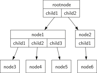
வரையறை இரண்டு: ஒரு மரம் காலியாக உள்ளது அல்லது வேர் மற்றும் பூஜ்ஜியத்தைக் கொண்டுள்ளது அல்லது பல துணை மரங்கள், அவை ஒவ்வொன்றும் ஒரு மரமாகும். ஒவ்வொரு துணை மரத்தின் வேர் ஒரு விளிம்பில் மூல மரத்தின் வேருடன் இணைக்கப்பட்டுள்ளது.
கீழே உள்ள வரைபடம் ஒரு மரத்தின் இந்த சுழல்நிலை வரையறையை விளக்குகிறது. ஒரு மரத்தின் சுழல்நிலை வரையறையைப் பயன்படுத்தி கீழே உள்ள மரத்தில் குறைந்தது நான்கு உச்சிகள் உள்ளது என்பதை நாம் அறிவோம். ஒரு துணை மரத்தை குறிக்கும் ஒவ்வொரு முக்கோணத்திற்கும் ஒரு வேர் இருக்க வேண்டும். அதில் பல உச்சிகள் இருக்கலாம், ஆனால் இது நாம் மரத்தை ஆழமாகப் பார்க்கவிடடால் தெரியாது.
A recursive definition of a tree
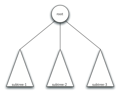
8.2 மரம் தரவமைப்பின் பிரதிநிதித்துவம் - Representing a Tree
இந்தப் பிரிவில், பைத்தானில் தரவு வகைகளுடன் மரம் போன்ற வடிவத்தைப் பிரதிநிதித்துவப்படுத்துவதற்கான சில வெவ்வேறு வழிகளைக் கருதுகிறோம். மரங்கள் பல சூழல்களில் நிகழ்கின்றன மற்றும் ஒன்றில் சரியான பிரதிநிதித்துவம் மற்றொன்றுக்கு பொருந்தாது என்பதால் பல பிரதிநிதித்துவங்களை நன்கு அறிந்திருப்பது முக்கியம்.
Python இல், html5lib அல்லது ast பைத்தானின் சுருக்க தொடரியல் இலக்கணத்துடன் பணிபுரிய) நாம் முதலில் விவாதிக்கும் உருப்படி சார்ந்த "உச்சிகள் மற்றும் குறிப்புகள்" பிரதிநிதித்துவத்தைப் பயன்படுத்தவும். எவ்வாறாயினும், எங்கள் சொந்த மரங்களைச் சுற்றி செயல்பாட்டைக் கட்டமைக்கும் போது, கட்டளைகள் மற்றும் பட்டியல்களிலிருந்து உருவாக்கப்பட்ட பிரதிநிதித்துவத்தைப் பயன்படுத்துவது பொதுவாக எளிதானது, அதை நாங்கள் பின்னர் விவாதிப்போம். இந்த எளிமையான பிரதிநிதித்துவம் மற்ற மொழிகள் மற்றும் சூழல்களுக்கு, உருப்படிகளைப் பற்றிய எண்ணம் இல்லாதவர்களுக்கும் (பேனா மற்றும் காகிதம் போன்றவை!) மிகவும் கையடக்கமானது.
உச்சிகள் மற்றும் குறிப்புக்களின் பிரதிநிதித்துவம்(Nodes and references representation)
ஒரு மரத்தைப் பிரதிநிதித்துவப்படுத்துவதற்கான எங்கள் முதல் முறையானது Node வகுப்பின் நிகழ்வுகளைப் முனை நிகழ்வுகளுக்கு இடையே உள்ள குறிப்புகளுடன் பயன்படுத்துகிறது
ஒரு சிறிய உதாரணத்தைப் பார்ப்போம்:
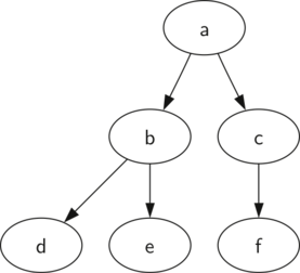
உச்சிகள் மற்றும் குறிப்புகளைப் பயன்படுத்தி, இந்த மரம் கட்டமைக்கப்பட்டவை போல் நாம் நினைக்கலாம்:
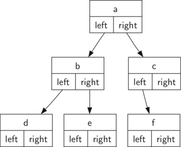
கீழே காட்டப்பட்டுள்ளபடி உச்சிகள் மற்றும் குறிப்புக்களின் அணுகுமுறைக்கான எளிய வகுப்பு வரையறையுடன் தொடங்குவோம். இந்த வழக்கில் நாம் இரு கிளை மரங்களைக் கருத்தில் கொள்வோம், எனவே left மற்றும் right உச்சிகளை நேரடியாகக் குறிப்பிடுவோம். கணுக்கள் இரண்டுக்கும் மேற்பட்ட குழந்தைகளைக் கொண்டிருக்கும் மரங்களுக்கு, அதற்குப் பதிலாக இந்தக் குறிப்புகளைக் கொண்டிருக்க children பட்டியலைப் பயன்படுத்தலாம்.
இந்தப் பிரதிநிதித்துவத்தைப் பற்றி நினைவில் கொள்ள வேண்டிய முக்கியமான விஷயம் என்னவென்றால், left மற்றும் right பண்புக்கூறுகள் Node வகுப்பின் மற்ற நிகழ்வுகளுக்கான குறிப்புகளாக மாறும். எடுத்துக்காட்டாக, மரத்தில் ஒரு புதிய இடது குழந்தையைச் செருகும்போது, Node இன் மற்றொரு நிகழ்வை உருவாக்கி, புதிய துணை மரத்தைக் குறிப்பிட வேரில் self.left ஐ மாற்றுவோம்.
class Node(object):
def __init__(self, val):
self.val = val
self.left = None
self.right = None
constructor செயல்பாடு முனையில் சேமிக்க சில வகையான மதிப்பைப் பெற எதிர்பார்க்கிறது என்பதைக் கவனியுங்கள்.நீங்கள் விரும்பும் எந்தப் உருப்படியையும் பட்டியலில் சேமித்து வைப்பது போல், val ஒரு முனைக்கான பண்புக்கூறு எந்த உருப்படிக்கும் ஒரு குறிப்பாக இருக்கலாம். எங்கள் ஆரம்ப உதாரணங்களுக்கு,உச்சியின் பெயரை மதிப்பாக சேமிப்போம். உச்சிகள் மற்றும் குறிப்புகளைப் பயன்படுத்தி மேலே விளக்கப்பட்டுள்ள மரத்தைப் பிரதிநிதித்துவப்படுத்தினால், Node வகுப்பின் ஆறு நிகழ்வுகளை உருவாக்குவோம்.
அடுத்து, வேர் உச்சிக்கு அப்பால் மரத்தை உருவாக்க உதவும் ஒரு செயல்பாட்டைப் பார்ப்போம். மரத்தில் இடது குழந்தையைச் சேர்க்க, நாங்கள் ஒரு புதிய Node நிகழ்வை நிறுவி, அதை இங்கே வரையறுக்கப்பட்டுள்ள insert_left செயல்பாட்டிற்கு child ஆக அனுப்புவோம்:
def insert_left(self, child):
if self.left is None:
self.left = child
else:
child.left = self.left
self.left = child
செருகுவதற்கு இரண்டு நிகழ்வுகளை நாம் கருத்தில் கொள்ள வேண்டும். ஏற்கனவே இல்லாத இடது குழந்தை இல்லாத உச்சியினால் முதல் வழக்கு வகைப்படுத்தப்படும்.இடது குழந்தை இல்லாதபோது, ஒரு உச்சியை மரத்திற்கு சேர்க்கவும். ஏற்கனவே உள்ள இடது குழந்தையின் உச்சியினால் இரண்டாவது வழக்கு வகைப்படுத்தப்படுகிறது.இரண்டாவது வழக்கில், நாம் ஒரு முனையைச் செருகி, மரத்தில் இருக்கும் குழந்தையை ஒரு நிலை கீழே தள்ளுகிறோம்.
insert_rightக்கான குறியீடு சமச்சீர் வழக்குகளின் தொகுப்பைக் கருத்தில் கொள்ள வேண்டும்.ஒன்று வலது குழந்தை இல்லை, அல்லது நாம் வேர் மற்றும் வலது குழந்தைக்கு இடையே ஒரு முனையை செருக வேண்டும்.
def insert_right(self, child): if self.right is None: self.right = child else: child.right = self.right self.right = child |
இப்போது இரு கிளை மரத்தை உருவாக்குவதற்கும் கையாளுவதற்கும் அனைத்து பகுதிகளும் எங்களிடம் உள்ளன, கட்டமைப்பை இன்னும் கொஞ்சம் சரிபார்க்க அவற்றைப் பயன்படுத்துவோம். முனை a வேராகக் கொண்டு ஒரு எளிய மரத்தை உருவாக்குவோம், மேலும் b மற்றும் c முனைகளை குழந்தைகளாகச் சேர்ப்போம். கீழே நாம் மரத்தை உருவாக்கி, key, left மற்றும் right புறத்தில் சேமிக்கப்பட்ட சில மதிப்புகளைப் பார்க்கிறோம். வேரின் இடது மற்றும் வலது குழந்தைகள் இருவரும் Node வகுப்பின் தனித்துவமான நிகழ்வுகளாக இருப்பதைக் கவனியுங்கள்.ஒரு மரத்திற்கான எங்கள் அசல் சுழல்நிலை வரையறையில் நாங்கள் கூறியது போல், இது ஒரு இரு கிளை மரத்தின் எந்தவொரு குழந்தையையும் இரு கிளை மரமாக கருத அனுமதிக்கிறது.
root = Node('a') root.val # => 'a' root.left # => None root.insert_left(Node('b')) root.left # => <__main__.Node object> root.left.val # => 'b' root.insert_right(Node('c')) root.right # => <__main__.Node object> root.right.val # => 'c' root.right.val = 'hello' root.right.val # => 'hello' |
பட்டியல்கள் பட்டியலின் பிரதிநிதித்துவம் (List of lists representation)
தூய தரவுகளைப் பயன்படுத்தி மரங்களை சுருக்கமாகப் பிரதிநிதித்துவப்படுத்துவதற்கான பொதுவான வழி பட்டியல்களின் பட்டியலாகும். பட்டியல்களின் பட்டியலில், ஒவ்வொரு உறுப்புக்கும் ஒரே ஒரு பெற்றோர் மட்டுமே (வெளிப்புற பட்டியல் வரை) இருப்பதால், சுழற்சிகள் இல்லாத படிநிலை அமைப்பாக ஒரு மரத்தைப் பற்றிய நமது எதிர்பார்ப்பைப் பூர்த்தி செய்கிறது.
பட்டியல்கள் மரத்தின் பட்டியலில், ஒவ்வொரு உச்சியின் மதிப்பையும் பட்டியலின் முதல் உறுப்பாக சேமிப்போம். பட்டியலின் இரண்டாவது உறுப்பு இடது துணை மரத்தைக் குறிக்கும் பட்டியலாக இருக்கும். பட்டியலின் மூன்றாவது உறுப்பு சரியான துணை மரத்தைக் குறிக்கும் மற்றொரு பட்டியலாக இருக்கும். இந்த நுட்பத்தை விளக்குவதற்கு, எங்கள் எடுத்துக்காட்டு மரத்தின் பட்டியல்களின் பட்டியலைப் பார்ப்போம்:
tree = [ 'a', #root [ 'b', # left subtree ['d' [], []], ['e' [], []] ], [ 'c', # right subtree ['f' [], []], [] ] ] |
நிலையான பட்டியல் அட்டவணையைப் பயன்படுத்தி பட்டியலின் துணை மரங்களை நாம் அணுகலாம் என்பதைக் கவனியுங்கள். மரத்தின் வேர் tree[0] ஆகும், வேரின் இடது துணை மரம் tree[1] ஆகும், வலது துணை மரம் tree[2] ஆகும். ஒரு பட்டியலைப் பயன்படுத்தி ஒரு எளிய மரத்தை உருவாக்குவதை கீழே விளக்குகிறோம். மரம் கட்டப்பட்டதும், நாம் வேர் மற்றும் இடது மற்றும் வலது துணை மரங்களை அணுகலாம்.
tree = ['a', ['b', ['d', [], []], ['e', [], []]], ['c', ['f', [], []], []]] # the left subtree tree[1] # => ['b', ['d', [], []], ['e', [], []]] # the right subtree tree[2] # => ['c', ['f', [], []], []] # the root tree[0] # => 'a' |
இந்த பட்டியல் அணுகுமுறையின் ஒரு நல்ல பண்பு என்னவென்றால், ஒரு துணை மரத்தைக் குறிக்கும் பட்டியலின் அமைப்பு ஒரு மரத்திற்கு வரையறுக்கப்பட்ட கட்டமைப்பை கடைபிடிக்கிறது; கட்டமைப்பே சுழல்நிலை ஆகும். வேர் மதிப்பு மற்றும் இரண்டு வெற்று பட்டியல்களைக் கொண்ட ஒரு துணை மரம் ஒரு இலை உச்சி ஆகும்.பட்டியல் அணுகுமுறையின் மற்றொரு நல்ல அம்சம் என்னவென்றால், இது பல துணை மரங்களைக் கொண்ட ஒரு மரத்திற்கு பொதுமைப்படுத்துகிறது. ஒரு இரு கிளை மரத்தை விட மரம் அதிகமாக இருந்தால், மற்றொரு துணை மரம் மற்றொரு பட்டியலாகும்.
இந்த பிரதிநிதித்துவம் வெறுமனே பட்டியல்களின் கலவையாக இருப்பதால், மேலே உள்ள எங்கள் உருப்படிகள் சார்ந்த "முனைகள் மற்றும் குறிப்புகள்" பிரதிநிதித்துவத்தில் உள்ள முறைகளுக்கு ஒப்பான ஒரு மரமாக கட்டமைப்பை கையாளுவதற்கு செயல்பாடுகளைப் பயன்படுத்துவோம்.
ஒரு மரத்தின் வேரில் இடது துணை மரத்தைச் சேர்க்க, வேர் பட்டியலின் இரண்டாவது நிலையில் புதிய பட்டியலைச் செருக வேண்டும். நாம் கவனமாக இருக்க வேண்டும். பட்டியலில் ஏற்கனவே இரண்டாவது நிலையில் ஏதாவது இருந்தால், அதைக் கண்காணித்து, நாம் சேர்க்கும் பட்டியலில் இடது குழந்தையாக மரத்தின் கீழே தள்ள வேண்டும். இடது குழந்தையைச் செருகுவதற்கான சாத்தியமான செயல்பாடு இங்கே:
def insert_left(root, child_val): subtree = root.pop(1) if len(subtree) > 1: root.insert(1, [child_val, subtree, []]) else: root.insert(1, [child_val, [], []]) return root |
இடது குழந்தையைச் செருக, நாம் முதலில் தற்போதைய இடது குழந்தையுடன் தொடர்புடைய பட்டியலைப் (வெறுமையாக இருக்கலாம்) பெறுவோம். நாங்கள் புதிய இடது குழந்தையைச் சேர்க்கிறோம், பழைய இடது குழந்தையை புதிய குழந்தையின் இடது குழந்தையாக நிறுவுகிறோம். எந்த நிலையிலும் மரத்தில் ஒரு புதிய உச்சியை பிரிக்க இது அனுமதிக்கிறது. insert_right க்கான நிரல் insert_left போலவே உள்ளது மற்றும் கீழே காட்டப்பட்டுள்ளது:
def insert_right(root, child_val): subtree = root.pop(2) if len(subtree) > 1: root.insert(2, [child_val, [], subtree]) else: root.insert(2, [child_val, [], []]) return root |
இந்த மரத்தை உருவாக்கும் செயல்பாடுகளின் தொகுப்பை முடிக்க, வேர் மதிப்பைப் பெறுவதற்கும் அமைப்பதற்கும், இடது அல்லது வலது துணை மரங்களைப் பெறுவதற்கும் இரண்டு அணுகல் செயல்பாடுகளை எழுதுவோம்.இடது துணை மரங்கள் மற்றும் வலது துணை மரங்களின் மதிப்புக்களைப் பிரதிநிதித்துவப்படுத்த பட்டியலில் உள்ள நிலைகளைப் பயன்படுத்துகிறோம் என்ற உண்மையை இந்த வழியில் சுருக்கலாம்:
def get_root_val(root): return root[0] def set_root_val(root, new_val): root[0] = new_val def get_left_child(root): return root[1] def get_right_child(root): return root[2] |
ஒரு மரத்தை உருவாக்கவும், கொடுக்கப்பட்ட உச்சிகளின் குழந்தைகளை மீட்டெடுக்கவும் இப்போது எங்கள் செயல்பாட்டு வரையறைகளைப் பயன்படுத்தலாம்:
root = [3, [], []] insert_left(root, 4) insert_left(root, 5) insert_right(root, 6) insert_right(root, 7) left = get_left_child(root) left # => [5, [4, [], []], []] set_root_val(left, 9) root # => [3, [9, [4, [], []], []], [7, [], [6, [], []]]] insert_left(left, 11) root # => [3, [9, [11, [4, [], []], []], []], [7, [], [6, [], []]]] get_right_child(get_right_child(root)) # => [6, [], []] |
விவரணையாக்கப் பிரதிநிதித்துவம் (Map-based representation)
எங்கள் பட்டியல் பிரதிநிதித்துவப் பட்டியலில் சில நன்மைகள் உள்ளன:
- இது சுருக்கமானது;
- நாம் எளிதாக மரத்தை பைதான் பட்டியல் எழுத்துக்களாக உருவாக்கலாம்;
- மரத்தை நாம் எளிதாக வரிசைப்படுத்தி அச்சிடலாம்; மற்றும்,
- உருப்படிகள் இல்லாத மொழிகள் மற்றும் சூழல்களுக்கு இது கையடக்கமானது.
எவ்வாறாயினும், ஒரு குறிப்பிட்ட வரியில் அச்சிடப்பட்டிருந்தால், அவற்றைப் பார்ப்பதன் மூலம், கூட்டுப் பட்டியல்களின் மரம் போன்ற இயல்பைப் பார்ப்பது சற்று கடினம் என்பது குறிப்பிடத்தக்க குறைபாடுகளைக் கொண்டுள்ளது.
இந்த காரணத்திற்காக, இந்த புத்தகத்தில் எங்கள் விருப்பம் (பெரும்பாலும் நிஜ வாழ்க்கை நிரலாக்கத்தில், அந்த விஷயத்தில்) உள்ளமை விவரணையாக்கத்தைப் பயன்படுத்தி (அதாவது பைத்தானில் உள்ள dict) மிகவும் ஒத்த பிரதிநிதித்துவத்தைப் பயன்படுத்துவதே ஆகும். மர முனை தொடர்பான பிற தரவு.
விவரணையாக்கத்தைப் பயன்படுத்தி, எங்கள் எடுத்துக்காட்டு மரம் இப்படி இருக்கலாம்:
{
'val': 'A',
'left': {
'val': 'B',
'left': {'val': 'D'},
'right': {'val': 'E'}
},
'right': {
'val': 'C',
'right': {'val': 'F'}
}
}
இந்த வழக்கில், எங்கள் ஒவ்வொரு முனையும் குறைந்தபட்சம் val சாவியுடன் விவரணையாக்கமாக மாறும், மேலும் சில சந்தர்ப்பங்களில் left மற்றும்/அல்லது right சாவி(கள்) ஆகும்.
இரு கிளை மரம் அல்லாத ஒரு மரத்தை நாம் கையாள்வது என்றால், அதற்குப் பதிலாக children சாவியைப் பயன்படுத்தலாம்:
{
'val': 'A',
'children': [
{
'val': 'B',
'children': [
{'val': 'D'},
{'val': 'E'},
]
},
{
'val': 'C',
'children': [
{'val': 'F'},
{'val': 'G'},
{'val': 'H'}
]
}
]
}
இது கிட்டத்தட்ட எங்களின் பட்டியல்களின் பிரதிநிதித்துவப் பட்டியலைப் போலவே கச்சிதமானது மற்றும் குறிப்பிடத்தக்கது மேலும் படிக்கக்கூடியது, எனவே இந்த விவரணையாக்க அடிப்படையிலான பிரதிநிதித்துவத்தை நாங்கள் புத்தகம் முழுவதும் தொடர்ந்து பயன்படுத்துவோம்.
8.3 பகுப்பாய்வு மரங்கள் - Parse Trees
எங்கள் மர தரவு கட்டமைப்பின் செயலாக்கம் முடிந்ததும்,சில உண்மையான பிரச்சனைகளை தீர்க்க ஒரு மரத்தை எவ்வாறு பயன்படுத்தலாம் என்பதற்கான உதாரணத்தை நாங்கள் இப்போது பார்க்கிறோம். இந்த பகுதியில் நாம் பாகுபடுத்தும் மரங்களைப் பார்ப்போம். பாகுபடுத்தும் மரங்களைப் பயன்படுத்தி வாக்கியங்கள் அல்லது கணிதம் போன்ற நிஜ உலக உதாரணங்களை பிரதிநிதித்துவப்படுத்துகிறது.
கீழே உள்ள வரைபடம் ஒரு எளிய வாக்கியத்தின் படிநிலை அமைப்பைக் காட்டுகிறது. ஒரு வாக்கியத்தை மர அமைப்பாகக் குறிப்பிடுவது, துணை மரங்களைப் பயன்படுத்தி வாக்கியத்தின் தனிப்பட்ட பகுதிகளுடன் வேலை செய்ய அனுமதிக்கிறது.
A parse tree for a simple sentence
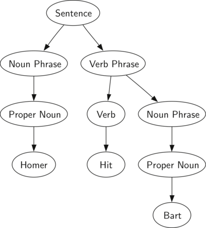
கீழே காட்டப்பட்டுள்ளபடி, ((7+3)×(5−2)) போன்ற ஒரு கணித வெளிப்பாட்டையும் நாம் பாகுபடுத்தும் மரமாகப் பிரதிநிதித்துவப்படுத்தலாம் முழு அடைப்புக் குறியிடப்பட்ட வெளிப்பாடுகளை நாங்கள் ஏற்கனவே பார்த்துள்ளோம், எனவே இந்த வெளிப்பாடு பற்றி நமக்கு என்ன தெரியும்? கூட்டல் அல்லது கழித்தல் இரண்டையும் விட பெருக்கல் அதிக முன்னுரிமை கொண்டது என்பதை நாம் அறிவோம்.அடைப்புக்குறிக்குள் இருப்பதால், பெருக்கல் செய்வதற்கு முன் அடைப்புக் கூட்டல் மற்றும் கழித்தல் வெளிப்பாடுகளை மதிப்பீடு செய்ய வேண்டும் என்பதை நாம் அறிவோம். மரத்தின் படிநிலை முழு வெளிப்பாட்டிற்கான மதிப்பீட்டின் வரிசையைப் புரிந்துகொள்ள உதவுகிறது. உயர்நிலைப் பெருக்கத்தை மதிப்பிடுவதற்கு முன், துணை மரங்களில் கூட்டல் மற்றும் கழித்தலை மதிப்பீடு செய்ய வேண்டும்.இடது துணை மரமாக இருக்கும் கூட்டல் 10 ஆக மதிப்பிடப்படுகிறது. வலது துணை மரமாக இருக்கும் கழித்தல் 3 ஆக மதிப்பிடப்படுகிறது. மரங்களின் படிநிலை அமைப்பைப் பயன்படுத்தி, உள்ள வெளிப்பாடுகளை மதிப்பீடு செய்தவுடன், குழந்தைகளில் ஒரு முழு துணை மரத்தையும் ஒரு உச்சியால் மாற்றலாம். இந்த மாற்று நடைமுறையைப் பயன்படுத்தினால், கீழே காட்டப்பட்டுள்ள எளிமையான மரத்தை நமக்கு வழங்குகிறது.
Parse tree for (7+3) * (5-2)
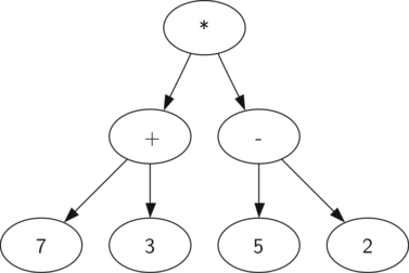
இந்த பகுதியின் எஞ்சிய பகுதியில் நாம் பாகுபடுத்தும் மரங்களை இன்னும் விரிவாக ஆராயப் போகிறோம். குறிப்பாக முழு அடைப்புக்குறியிடப்பட்ட கணித வெளிப்பாட்டிலிருந்து ஒரு பாகுபடுத்தும் மரத்தை எவ்வாறு உருவாக்குவது மற்றும் ஒரு பாகுபடுத்தப்பட்ட மரத்தில் சேமிக்கப்பட்ட வெளிப்பாட்டை எவ்வாறு மதிப்பிடுவது என்பதைப் பார்ப்போம்.
பாகுபடுத்தும் மரத்தை உருவாக்குவதற்கான முதல் படி, வெளிப்பாடு சரத்தை டோக்கன்களின் பட்டியலாகப் பிரிப்பதாகும். கருத்தில் கொள்ள நான்கு வெவ்வேறு வகையான டோக்கன்கள் உள்ளன: இடது அடைப்புக்குறிகள், வலது அடைப்புக்குறிப்புகள், இயக்கங்கள் மற்றும் செயல்பாடுகள்.நாம் ஒரு இடது அடைப்புக்குறியைப் படிக்கும்போதெல்லாம் ஒரு புதிய வெளிப்பாட்டைத் தொடங்குகிறோம் என்பதை நாம் அறிவோம், எனவே அந்த வெளிப்பாட்டிற்கு ஏற்ப ஒரு புதிய மரத்தை உருவாக்க வேண்டும். மாறாக, வலது அடைப்புக்குறியைப் படிக்கும்போதெல்லாம், ஒரு வெளிப்பாட்டை முடித்திருக்கிறோம்.operands கள் இலை உச்சிகளாகவும் , அவற்றை இயக்குபவர்களின் குழந்தைகளாகவும் இருக்கும் என்பதையும் நாங்கள் அறிவோம். இறுதியாக, ஒவ்வொரு ஆபரேட்டருக்கும் இடது மற்றும் வலது குழந்தை இருக்கப் போகிறது என்பதை நாங்கள் அறிவோம்.
மேலே உள்ள தகவலைப் பயன்படுத்தி, நான்கு விதிகளை பின்வருமாறு வரையறுக்கலாம்:
A simplified parse tree for (7+3) * (5-2)
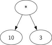
இந்த பகுதியின் எஞ்சிய பகுதியில் நாம் பாகுபடுத்தும் மரங்களை இன்னும் விரிவாக ஆராயப் போகிறோம். குறிப்பாக முழு அடைப்புக்குறியிடப்பட்ட கணித வெளிப்பாட்டிலிருந்து ஒரு பாகுபடுத்தும் மரத்தை எவ்வாறு உருவாக்குவது மற்றும் ஒரு பாகுபடுத்தப்பட்ட மரத்தில் சேமிக்கப்பட்ட வெளிப்பாட்டை எவ்வாறு மதிப்பிடுவது என்பதைப் பார்ப்போம்.
பாகுபடுத்தும் மரத்தை உருவாக்குவதற்கான முதல் படி, வெளிப்பாடு சரத்தை டோக்கன்களின் பட்டியலாகப் பிரிப்பதாகும். கருத்தில் கொள்ள நான்கு வெவ்வேறு வகையான டோக்கன்கள் உள்ளன: இடது அடைப்புக்குறிகள், வலது அடைப்புக்குறிப்புகள், இயக்கங்கள் மற்றும் செயல்பாடுகள்.நாம் ஒரு இடது அடைப்புக்குறியைப் படிக்கும்போதெல்லாம் ஒரு புதிய வெளிப்பாட்டைத் தொடங்குகிறோம் என்பதை நாம் அறிவோம், எனவே அந்த வெளிப்பாட்டிற்கு ஏற்ப ஒரு புதிய மரத்தை உருவாக்க வேண்டும். மாறாக, வலது அடைப்புக்குறியைப் படிக்கும்போதெல்லாம், ஒரு வெளிப்பாட்டை முடித்திருக்கிறோம்.operands கள் இலை உச்சிகளாகவும் , அவற்றை இயக்குபவர்களின் குழந்தைகளாகவும் இருக்கும் என்பதையும் நாங்கள் அறிவோம். இறுதியாக, ஒவ்வொரு ஆபரேட்டருக்கும் இடது மற்றும் வலது குழந்தை இருக்கப் போகிறது என்பதை நாங்கள் அறிவோம்.
மேலே உள்ள தகவலைப் பயன்படுத்தி, நான்கு விதிகளை பின்வருமாறு வரையறுக்கலாம்
- தற்போதைய டோக்கன் '(') எனில், இடது குழந்தையாக புதிய உச்சியை சேர்க்கவும்.தற்போதைய முனை, மற்றும் இடது குழந்தைக்கு இறங்குகிறது.
- தற்போதைய டோக்கன் ['+','-','/','*'] பட்டியலில் இருந்தால், தற்போதைய டோக்கன் ஆல் பிரதிநிதித்துவப்படுத்தப்படும் ஆபரேட்டருக்கான தற்போதைய உச்சியின் வேர் மதிப்பாக அமைக்கவும்.தற்போதைய முனையின் வலது குழந்தையாக புதிய முனையைச் சேர்க்கவும் மற்றும் வலது குழந்தைக்கு இறங்குங்கள்.
- தற்போதைய டோக்கன் ஒரு எண்ணாக இருந்தால், அந்த எண்ணுக்கு தற்போதைய உச்சியின் வேர் மத்திப்பை அமைப்பதோடு பெற்றோரிடம் திரும்பவும்.
- தற்போதைய டோக்கன் ')'' எனில், தற்போதைய முனையின் பெற்றோருக்குச் செல்லவும்.
பைதான் நிரலை எழுதுவதற்கு முன், விதிகளின் உதாரணத்தைப் பார்ப்போம் செயலில் மேலே கோடிட்டுக் காட்டப்பட்டுள்ளது. (3 + (4 x 5)) என்ற வெளிப்பாட்டைப் பயன்படுத்துவோம். நாங்கள் பின்வரும் ['(', '3', '+', '(', '4', '*', '5' ,')',')'] எழுத்துக்குறி டோக்கன்களின் பட்டியலில் இந்த வெளிப்பாட்டைப் பாகுபடுத்தும். ஆரம்பத்தில் நாம் ஒரு வெற்று வேர் உச்சியை கொண்ட ஒரு பாகுபடுத்தும் மரத்துடன் தொடங்கவும். பாகுபடுத்தும் மரத்தின், ஒவ்வொரு புதிய டோக்கனும் செயலாக்கப்படும் போது கீழே உள்ள புள்ளிவிவரங்கள் கட்டமைப்பு மற்றும் உள்ளடக்கங்களை விளக்குகின்றன

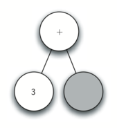
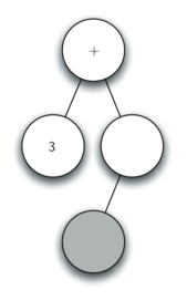
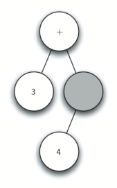
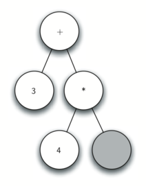
Tracing parse tree construction
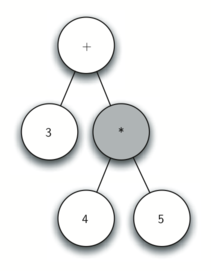
மேலே உள்ளவற்றைப் பயன்படுத்தி, உதாரணத்தின் மூலம் படி படியாக நடப்போம்:
- வெற்று மரத்தை உருவாக்கவும்.
- ( இனை முதல் டோக்கனாகப் படிக்கவும். விதி 1ன்படி, வேரின் இடது குழந்தையாக புதிய உச்சியை உருவாக்கவும் தற்போதைய உச்சியை இந்தப் புதிய குழந்தையாக மாற்றவும்.
- அடுத்த டோக்கனாக 3ஐப் படியுங்கள். விதி 3 மூலம், வேர் மதிப்பை தற்போதைய முனை 3 ஆகவும் அமைக்கவும் மற்றும் மரத்தின் பெற்றோரிடம் செல்லவும்.
- அடுத்த டோக்கனாக + படிக்கவும். விதி 2 மூலம், வேர் மதிப்பை அமைக்கவும் தற்போதைய முனை + க்கு மற்றும் வலது குழந்தையாக புதிய முனையைச் சேர்க்கவும். புதிய வலது குழந்தை தற்போதைய முனை ஆகிறது.
- ( இனை அடுத்த டோக்கனாக. விதி 1 இன் படி, தற்போதைய உச்சியின் இடது குழந்தையாக ஒரு புதிய முனையை உருவாக்கவும்.தற்போதைய முனையின் குழந்தை. புதிய இடது குழந்தை ஆகிறது
- அடுத்த டோக்கனாக 4 ஐப் படியுங்கள். விதி 3 மூலம், தற்போதைய உச்சிக்கு 4 மதிப்பை அமைக்கவும் . 4 இன் பெற்றோரை தற்போதைய முனையாக மாற்றவும்.
- அடுத்த டோக்கனாக * படிக்கவும். விதி 2 மூலம், வேர் மதிப்பை தற்போதைய முனை * இற்கு அமைக்கவும் மற்றும் ஒரு புதிய வலது குழந்தை உருவாக்க. புதிய வலது குழந்தை தற்போதைய முனையாக மாறும்.
- அடுத்த டோக்கனாக 5 ஐப் படியுங்கள். விதி 3 மூலம், வேர் மதிப்பை தற்போதைய முனை 5 ஆக அமைக்கவும் . 5 இன் பெற்றோரை தற்போதைய முனையாக மாற்றவும்.
- அடுத்த டோக்கனாக ) படிக்கவும். விதி 4 மூலம் நாம் * வின் பெற்றோராக தற்போதைய முனையை ஆக்குகிறோம்
- அடுத்த டோக்கனாக ) படிக்கவும். விதி 4 மூலம் நாம்தற்போதைய முனை+ இந்த பெற்றோராக்கின்றோம் . இந்த கட்டத்தில் + க்கு பெற்றோர் இல்லை, எனவே நாங்கள் முடித்துவிட்டோம்.
மேலே உள்ள உதாரணத்திலிருந்து, தற்போதைய உச்சி மற்றும் தற்போதைய உச்சியின் பெற்றோரை நாம் கண்காணிக்க வேண்டும் என்பது தெளிவாகிறது.எளிய தீர்வு நாம் மரத்தை கடக்கும்போது பெற்றோரின் தடம் ஒரு அடுக்கைப் பயன்படுத்துவதாகும். நாம் எப்போது வேண்டுமானாலும் தற்போதைய உச்சியின் குழந்தைக்கு இறங்க, நாம் முதலில் தற்போதைய உச்சியை இயக்குகிறோம் தற்போதைய முனையின் பெற்றோருக்குத் திரும்ப விரும்பினால், நாங்கள் பெற்றோர் அடுக்கிலிருந்து வெளியே எடுக்கின்றோம்
அடுக்கு மற்றும் இருகிளை மரத்தின் சுருக்கத் தரவு வகைகள் மேலே விவரிக்கப்பட்ட விதிகளைப் பயன்படுத்துதல், நாம் இப்போது ஒரு பாகுபடுத்தும் மரத்தை உருவாக்க பைதான் செயல்பாட்டை எழுத தயாராக உள்ளோம்.. எங்கள் பாகுபடுத்
தும் மரத்தை உருவாக்குவதற்கான நிரல் கீழே கொடுக்கப்பட்டுள்ளது.
import operator OPERATORS = { '+': operator.add, '-': operator.sub, '*': operator.mul, '/': operator.truediv } LEFT_PAREN = '(' RIGHT_PAREN = ')' def build_parse_tree(expression): tree = {} stack = [tree] node = tree for token in expression: if token == LEFT_PAREN: node['left'] = {} stack.append(node) node = node['left'] elif token == RIGHT_PAREN: node = stack.pop() elif token in OPERATORS: node['val'] = token node['right'] = {} stack.append(node) node = node['right'] else: node['val'] = int(token) parent = stack.pop() node = parent return tree |
The four rules for building a parse tree are coded as the four clauses of the if statement above. In each case you can see that the code implements the rule.
Now that we have built a parse tree, we can write a function to evaluate it, returning the numerical result. To write this function, we will make use of the hierarchical nature of the tree to write an algorithm that evaluates a parse tree by recursively evaluating each subtree.
A natural base case for recursive algorithms that operate on trees is to check for a leaf node. In a parse tree, the leaf nodes will always be operands. Since numerical objects like integers and floating points require no further interpretation, the evaluate function can simply return the value stored in the leaf node. The recursive step that moves the function toward the base case is to call evaluate on both the left and the right children of the current node. The recursive call effectively moves us down the tree, toward a leaf node.
To put the results of the two recursive calls together, we can simply apply the operator stored in the parent node to the results returned from evaluating both children. In the example from above we see that the two children of the root evaluate to themselves, namely 10 and 3. Applying the multiplication operator gives us a final result of 30.
The code for a recursive evaluate function is shown below. First, we obtain references to the left and the right children of the current node. If both the left and right children evaluate to None, then we know that the current node is really a leaf node. If the current node is not a leaf node, look up the operator in the current node and apply it to the results from recursively evaluating the left and right children.
To implement the arithmetic, we use a dictionary with the keys '+', '-', '*', and '/'. The values stored in the dictionary are functions from Python’s operator module. The operator module provides us with the functional versions of many commonly used operators. When we look up an operator in the dictionary, the corresponding function object is retrieved. Since the retrieved object is a function, we can call it in the usual way function(param1, param2). So the lookup OPERATORS['+'](2, 2) is equivalent to operator.add(2, 2).
def evaluate(tree): try: operate = OPERATORS[tree['val']] return operate(evaluate(tree['left']), evaluate(tree['right'])) except KeyError: # no left or no right, so is a leaf - our base case return tree['val'] |
Finally, we will trace the evaluate function on the parse tree we created above. When we first call evaluate, we pass the root of the entire tree as the parameter parse_tree. Then since the left and right children exist, we look up the operator in the root of the tree, which is '+', and which maps to the operator.add function. As usual for a Python function call, the first thing Python does is to evaluate the parameters that are passed to the function. In this case both parameters are recursive function calls to our evaluate function. Using left-to-right evaluation, the first recursive call goes to the left. In the first recursive call the evaluate function is given the left subtree. We find that the node has no left or right children, so we are in a leaf node. When we are in a leaf node we just return the value stored in the leaf node as the result of the evaluation. In this case we return the integer 3.
At this point we have one parameter evaluated for our top-level call to operator.add. But we are not done yet. Continuing the left-to-right evaluation of the parameters, we now make a recursive call to evaluate the right child of the root. We find that the node has both a left and a right child so we look up the operator stored in this node, '*', and call this function using the left and right children as the parameters. At this point you can see that both recursive calls will be to leaf nodes, which will evaluate to the integers four and five respectively. With the two parameters evaluated, we return the result of operator.mul(4, 5). At this point we have evaluated the operands for the top level '+' operator and all that is left to do is finish the call to operator.add(3, 20). The result of the evaluation of the entire expression tree for (3+(4×5))(3 + (4 x 5))(3+(4×5)) is 23.
8.4 மரம் தரவமைப்பு பயணித்தல் - Tree Traversals
இப்போது எங்கள் மர தரவுகளின் அடிப்படை கட்டமைப்பு செயல்பாட்டை ஆய்வு செய்துள்ளோம். மரங்களின் சில கூடுதல் பயன்பாட்டு முறைகளைப் பார்க்க வேண்டிய நேரம் இது மரங்களின் உச்சிகளை அணுகுவதன் அடிப்படையில் இந்த பயன்பாட்டு முறைகளை நாம் மூன்று வழிகளாகப் பிரிக்கலாம்.பொதுவாகப் பயன்படுத்தப்படும் மூன்று வடிவங்கள் உள்ளன.ஒரு மரத்தில் உள்ள அனைத்து உச்சிகளையும் பார்வையிடவும். பார்வையிட்ட இந்த உச்சிகளுக்கு இடையிலான வேறுபாடு தொடர்பு ஒரு வரிசையானதாகும்.இந்த உச்சிகளை பார்வையிடும் செயற்பாட்டை நாங்கள் “traversal.” என அழைக்கின்றோம்.உச்சிகளை பார்வையிடும் இந்த மூன்று செயற்பாடுகளையும் நாம் preorder, inorder, மற்றும் postorder. என அழைக்கின்றோம். இந்த மூன்று பயணங்களை இன்னும் கவனமாக வரையறுத்து, சிலவற்றைப் பாருங்கள் இந்த வடிவங்கள் பயனுள்ளதாக இருக்கும் உதாரணங்கள் மூலம் ஆரம்பிக்கலாம்..
மூன்கூட்டிய-சீர்வழி (preorder): முன்கூட்டிய ஒழுங்குபடுத்தப்பட்ட பயணத்தில், முதலில் வேர் உச்சியைப் பார்வையிடுவோம்.பின்னர் சுழல்நிலையாக இடது துணை மரத்தில் முன்கூட்டிய ஒழுங்குபடுத்தப்பட்ட பயணத்தை செய்யவும், அதைத் தொடர்ந்து வலது துணை மரத்தில் ஒரு சுழல்நிலையாக முன்கூட்டிய ஒழுங்குபடுத்தப்பட்ட பயணத்தை செய்யவும்.
சீர்வழி (inorder): ஒரு ஒழுங்கற்ற பயணத்தில், இடது துணைமரத்தில் ஒரு ஒழுங்கற்ற பயணத்தை நாங்கள் செய்கிறோம், வேர் உச்சியைப் பார்வையிடுகிறோம், இறுதியாக வலது துணை மரத்தில் சுழல்நிலை வரிசைப் பயணம் செய்கிறோம்.
பின்-சீர்வழி(postorder): ஒரு பின் திட்டமிட்ட பயணத்தில் , இடது துணைமரம் மற்றும் வலது துணை மரத்தின் பின் திட்டமிட்ட பயணத்தை சுழல்முறையில் செய்கிறோம், அதைத் தொடர்ந்து வேர் உச்சியைப் பார்வையிடுவோம்.
இந்த மூன்று வகையான பயணங்கள் ஒவ்வொன்றையும் விளக்கும் சில உதாரணங்களைப் பார்ப்போம். முதலில் முன்கூட்டிய ஒழுங்குபடுத்தப்பட்ட பயணத்தைப் பார்ப்போம்.ஒரு உதாரணமாக ஒரு மரத்தில் பயணிக்க, இந்த புத்தகத்தை ஒரு மரமாக பிரதிநிதித்துவப்படுத்துவோம். புத்தகம் மரத்தின் வேர் ஆகும். ஒவ்வொரு அத்தியாயமும் வேரின் குழந்தை.ஒரு அத்தியாயத்தில் உள்ள பகுதி ஒவ்வொன்றும் அத்தியாயத்தின் குழந்தை, மற்றும் ஒவ்வொரு துணைப்பிரிவும் அதன் பிரிவின் குழந்தை, மற்றும் பல. கீழேயுள்ள வரைபடம் இரண்டு அத்தியாயங்களைக் கொண்ட புத்தகத்தின் வரையறுக்கப்பட்ட பதிப்பைக் காட்டுகிறது.பயணிக்கும் வழிமுறை எத்தனை குழந்தைகளைக் கொண்ட மரங்களுக்கு வேலை செய்கிறது என்பதை கவனிக்கவும், ஆனால் நாங்கள் இப்போதைக்கு இரு கிளை மரங்களுடன் பயணிப்போம்.
Representing a book as a tree
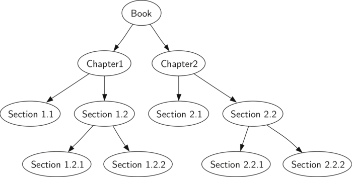
நீங்கள் இந்தப் புத்தகத்தை முன்னும் பின்னும் படிக்க விரும்புகிறீர்கள் என்று வைத்துக்கொள்வோம்.முன்கூட்டிய ஒழுங்குபடுத்தப்பட்ட பயணித்தல் உங்களுக்கு அந்த வரிசையை சரியாக வழங்குகிறது.மரத்தில் (புத்தக உச்சி ) நாம் முன்கூட்டிய ஒழுங்குபடுத்தப்பட்ட பயணித்தலைப் பின்பற்றுவோம் அறிவுறுத்தல்கள் வேரிலிருந்து தொடங்குகிறது. வழக்கு அத்தியாயம் 1 இல், இடது பக்கத்தில் உள்ள preorder என்பதை சுழல் முறையில் அழைக்கிறோம்.பிரிவு 1.1 ஐப் பெறுவதற்காக இடது குழந்தையில் preorder மீண்டும் சுழல் முறையில் அழைக்கின்றோம்.இருப்பினும் பிரிவு 1.1 இல் குழந்தைகள் இல்லாததால் கூடுதல் சுழல் அழைப்புக்களை நாங்கள் மேற்கொள்ளவில்லை.பிரிவு 1.1 ஐ முடித்த பின்னர் அத்தியாயம் 1 இற்கு மரத்தினை நகர்த்துவோம்.இந்த நிலையில் நாங்கள் இப்போதும் அத்தியாயம் 1 இன் வலது துணைமரத்திற்குப் பயணிக்க வேண்டும்.இது பிரிவு 1.2 ஆகும்.முன்னர் நாங்கள் இடது துணை மரத்திற்குப் பயணித்த போது அது பிரிவு 1.2.1 ஐ எங்களுக்கு வழங்கியது.பின்னர் நாங்கள் பிரிவு 1.2.2 இற்காக உச்சிக்குப் பயணிக்கும் போது பிரிவு 1.2 நிறைவடைகின்றது.அத்தோடு நாங்கள் அத்தியாயம் 1 இற்கு திரும்புவோம்.பின்னர் நாங்கள் மீண்டும் புத்தக உச்சிக்கு திரும்பி இதே படிமுறைகளை அத்தியாயம் 2 திற்காக பின்பற்றுவோம்.
மரப் பயணங்களை எழுதுவதற்கான நிரலாக்கம் வியக்கத்தக்க வகையில் நேர்த்தியாக உள்ளது, பெரும்பாலும் பயணங்கள் சுழல்நிலையில் எழுதப்பட்டிருப்பதால். கீழே உள்ள நிரலாக்கம் ஒரு இரு கிளை மரத்தின் முன்கூட்டிய ஒழுங்குபடுத்தப்பட்ட பயணத்தின் எளிய பைதான் செயல்படுத்தல் ஆகும். இந்த அணுகுமுறை குறிப்பாக நேர்த்தியானது, ஏனென்றால் எங்கள் அடிப்படை வழக்கு மரம் இருக்கிறதா என்று சரிபார்க்க வேண்டும். மர செயலுருபு None எனில், செயல்பாடு எந்த நடவடிக்கையும் எடுக்காமல் திரும்பும்.
def preorder(node):
if node:
print(node['val'])
preorder(node.get('left'))
preorder(node.get('right'))
கீழே காட்டப்பட்டுள்ள postorder ஆனது பயணித்தலுக்கான வழிமுறையின் preorder க்கு கிட்டத்தட்ட ஒத்ததாக உள்ளது.தவிர, அழைப்பை அச்சிடுவதற்கான செயல்பாட்டின் இறுதிக்கு நகர்த்துவோம்.
def postorder(node):
if node:
postorder(node.get('left'))
postorder(node.get('right'))
print(node['val'])
முன்கூட்டிய ஒழுங்குபடுத்தப்பட்ட பயணித்தலின் பொதுவான பயன்பாட்டை நாங்கள் ஏற்கனவே பார்த்தோம், அதாவது ஒரு பாகுபடுத்தப்பட்ட மரத்தை மதிப்பீடு செய்தல். பாடுபடுத்தும் மரத்தை மதிப்பீடு செய்வதற்கு முன்னைய அத்தியாயத்தில் என்ன செய்தோம்? இடது துணை மரத்தை மதிப்பீடு செய்தல் , வலது துணை மரத்தை மதிப்பீடு செய்தல் பின்னர் வேரில் இயக்கும் செயற்பாட்டை அழைப்பதன் மூலம் இரண்டையும் ஒன்று சேர்த்தலாகும்.
இந்தப் பகுதியில் நாம் பார்க்கப்போகும் இறுதிப் பயணமானது ஒழுங்கமைக்கப்பட்ட பயணமாகும். ஒழுங்கான பயணத்தில் நாம் இடது துணை மரத்தையும், அதைத் தொடர்ந்து வேரையும், இறுதியாக வலது துணை மரத்தையும் பார்வையிடுகிறோம். மூன்று பயணித்தல் செயல்பாடுகளிலும், இரண்டு சுழல்நிலை செயல்பாடு அழைப்புகளைப் பொறுத்து print அறிக்கையின் நிலையை மாற்றுகிறோம் என்பதைக் கவனியுங்கள்.
def inorder(node):
if node:
inorder(node.get('left'))
print(node['val'])
inorder(node.get('right'))
நாம் ஒரு பாகுபடுத்தும் மரத்தில் ஒரு எளிய வரிசைப் பயணத்தை மேற்கொண்டால், நம்முடைய அசல் வெளிப்பாட்டை மீண்டும் பெறுவோம். அடைப்புக்குறிகள் இல்லாமல்,முழு அடைப்புக்குறிக்குள் மீட்டமைக்க எங்களை அனுமதிக்கும் அடிப்படை ஒழுங்கற்ற வழிமுறையின் வெளிப்பாட்டின் பாதிப்பை மாற்றியமைப்போம். அடிப்படை டெம்ப்ளேட் இல் நாம் செய்யும் மாற்றங்கள் பின்வருமாறு: இடது அடைப்புக்குறியை இடது துணை மரத்தின் சுழல் அழைப்புக்கு (முன் ) before அச்சிடவும்.வலது அடைப்புக்குறியை வலது துணை மரத்தின் சுழல் அழைப்புக்கு (பின்) after அச்சிடவும். மாற்றியமைக்கப்பட்ட நிரலாக்கம் கீழே காட்டப்பட்டுள்ளது.
def construct_expression(parse_tree):
if parse_tree is None:
return ''
left = construct_expression(parse_tree.get('left'))
right = construct_expression(parse_tree.get('right'))
val = parse_tree['val']
if left and right:
return '({}{}{})'.format(left, val, right)
return val
8.5 Priority Queues with Binary Heaps
வரிசையின் ஒரு முக்கியமான மாறுபாடு முன்னுரிமை வரிசை ஆகும். ஒரு முன்னுரிமை வரிசை ஒரு வரிசையைப் போல் செயல்படுகிறது.இருப்பினும், முன்னுரிமை வரிசையில் ஒரு வரிசையில் உள்ள உருப்படிகளின் தருக்க வரிசை அவர்களின் "முன்னுரிமை" மூலம் தீர்மானிக்கப்படுகிறது. குறிப்பாக, அதிக முன்னுரிமை உருப்படிகள் குறைந்த முன்னுரிமை உருப்படிகளுக்கு முன்னால் வரிசையில் இருந்து வெளியே எடுக்கப்பட்டது.
முன்னுரிமை வரிசையானது குறிப்பிட்ட ஒரு பயனுள்ள தரவுக் கட்டமைப்பாக Dijkstra இன் குறுகிய பாதை வழிமுறை போன்ற வழிமுறைகள் போல் இருப்பதைப் பார்ப்போம்.இன்னும் பொதுவாக, முன்னுரிமை வரிசைகள் போதுமான அளவு பயனுள்ளதாக இருக்கும், நீங்கள் ஏற்கனவே ஒன்றை சந்தித்திருக்கலாம்: உதாரணமாக செய்தி வரிசைகள் அல்லது பணிகளின் வரிசைகள் பொதுவாக சில உருப்படிகளுக்கு மற்றயவற்றை விட முன்னுரிமை அளிக்கின்றன.
வரிசைப்படுத்துதல் செயல்பாடுகள் மற்றும் வரிசைகள் அல்லது பட்டியல்களைப் பயன்படுத்தி முன்னுரிமை வரிசையைச் செயல்படுத்துவதற்கான இரண்டு எளிய வழிகளைப் பற்றி நீங்கள் சிந்திக்கலாம். இருப்பினும், பட்டியலை வரிசைப்படுத்துவது O(n log[n]) ஆகும். நாம் சிறப்பாக செய்ய முடியும்.
முன்னுரிமை வரிசையை செயல்படுத்துவதற்கான உன்னதமான வழி இருபடி குவியல்(binary heap) எனப்படும் தரவு கட்டமைப்பைப் பயன்படுத்துவதாகும்.இருபடி குவியல் தரவுக் கட்டமைப்பானது O(log{n}) உருப்படிகளை வரிசைப்படுத்த அல்லது வரிசைப்படுத்த நம்மை அனுமதிக்கும்.
இருபடிக் குவியல் பற்றி கற்பது சுவாரஸ்யமானது, ஏனென்றால் குவியல்களை வரைபடமாக்கும்போது அது ஒரு மரமாகத் தெரிகிறது, ஆனால் அதைச் செயல்படுத்தும்போது அதன் உள் பிரதிநிதித்துவமாக ஒரு மாறும் வரிசையை (பைத்தான் பட்டியல் போன்றவை) மட்டுமே பயன்படுத்துகிறோம். இருபடிக் குவியல் இரண்டு பொதுவான மாறுபாடுகளைக் கொண்டுள்ளது: நிமிடக் குவியல், இதில் சிறிய விசை எப்போதும் முன்பக்கத்தில் இருக்கும், மற்றும் அதிகபட்சக் குவியல், இதில் மிகப்பெரிய விசை மதிப்பு எப்போதும் முன்பக்கத்தில் இருக்கும். இந்த பிரிவில் நாம் min heap ஐ செயல்படுத்துவோம், ஆனால் max heap அதே வழியில் செயல்படுத்தப்படுகிறது.
எங்கள் இருபடி குவியலுக்கு நாங்கள் செயல்படுத்தும் அடிப்படை செயல்பாடுகள்:
- BinaryHeap() புதிய, வெற்று, இருபடிக் குவியலை உருவாக்குகிறது.
- insert(k) குவியலில் ஒரு புதிய உருப்படியை சேர்க்கிறது.
- find_min() குவியலில் உள்ள பொருள் குறைந்தபட்ச முக்கிய மதிப்புடன் உருப்படியைத் திருப்பி, வெளியேறும்
- del_min() குவியல் இருந்து உருப்படியை அகற்றி, குறைந்தபட்ச முக்கிய மதிப்புடன் உருப்படியை வழங்குகிறது.
- is_empty() குவியல் காலியாக இருந்தால் true , இல்லையெனில் false என்று திரும்பும்.
- size() குவியலில் உள்ள பொருட்களின் எண்ணிக்கையை வழங்குகிறது.
- build_heap(list) சாவிகளின் பட்டியலிலிருந்து ஒரு புதிய குவியலை உருவாக்குகிறது.
(கட்டமைப்பு சொத்து) The Structure Property
எங்கள் குவியல் திறமையாக செயல்பட, நாங்கள் நமது குவியலைக் குறிக்கும்.இருகிளை மரத்தின் மடக்கைத் தன்மையை பயன்படுத்திக்கொள்வோம்.மடக்கை செயல்திறனுக்கு உத்தரவாதம் அளிக்க, நாம் நமது மரத்தை சமச்சீராக வைத்திருக்க வேண்டும் ஒரு சமச்சீர் இருகிளை மரம் தோராயமாக வேரின் இடது மற்றும் வலது துணை மரங்களில் சம எண்ணிக்கையிலான உச்சிகளைக் கொண்டுள்ளது.எங்கள் குவியல் செயல்படுத்தலில் நாம் முழுமையான இருகிளை மரத்தை உருவாக்குவதன் மூலம் மரத்தை சமநிலையில் வைத்திருங்கள்.முழுமையான இருகிளை மரம் என்பது ஒவ்வொரு மட்டத்திலும் அதன் அனைத்து உச்சிகளையும் கொண்டிருக்கும் ஒரு மரத்தில் இதற்கு விதிவிலக்கு மரத்தின் கீழ் மட்டமாகும், அதை நாம் இடமிருந்து வலம் நிரப்புகிறோம். இந்த வரைபடம் ஒரு முழு இருகிளை மரத்தின் உதாரணத்தைக் காட்டுகிறது:
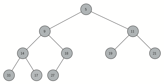
ஒரு முழுமையான மரத்தின் மற்றொரு சுவாரஸ்யமான சொத்து என்னவென்றால், அதை நாம் ஒற்றை பட்டியலைப் பிரதிநிதித்துவப்படுத்த பயன்படுத்த முடியும். நாம் உச்சிகள் மற்றும் குறிப்புகள் அல்லது பட்டியல்களின் பட்டியல்களைப் பயன்படுத்த வேண்டியதில்லை. மரம் முழுமையடைந்ததால், பெற்றோரின் இடது குழந்தை (நிலையில் p) என்பது பட்டியலில் 2p நிலையில் காணப்படும் உச்சி ஆகும். இதேபோல், பெற்றோரின் வலது குழந்தை பட்டியலில் 2p + 1 நிலையில் உள்ளது.மரத்தில் உள்ள எந்த உச்சியினதும் பெற்றோரைக் கண்டுபிடிக்க, நாம் வெறுமனே முழு எண் பிரிவைப் பயன்படுத்தலாம் (இயல்பானது போல கணிதப் பிரிவு தவிர மீதியை நிராகரிக்கிறோம்). ஒரு முனை உள்ளது என்று கொடுக்கப்பட்ட பட்டியலில் n நிலை, பெற்றோர் n/2 நிலையில் உள்ளார்.
கீழே உள்ள வரைபடம் ஒரு முழுமையான இரு கிளை மரத்தைக் காட்டுகிறது மற்றும் பட்டியலையும் தருகிறது மரத்தின் பிரதிநிதித்துவம். 2p மற்றும் 2p+1 பெற்றோர் மற்றும் குழந்தைகள்இடையே உள்ள தொடர்பைக் கவனியுங்கள். மரத்தின் பட்டியல் பிரதிநிதித்துவமானது , முழுமையான கட்டமைப்பு சொத்து, ஒரு முழுமையான இரு கிளை மரத்தை திறமையாக பயணிக்க அனுமதிப்பதோடு சில எளிய கணித செயல்பாடுகளை மட்டுமே பயன்படுத்துகிறது.எங்கள் இருபடி குவியலை திறம்பட செயல்படுத்த வழிவகுக்கிறது நாம் இதையும் பார்ப்போம்.
குவியல் வரிசை அம்சம் - The Heap Order Property
குவியலில் உருப்படிகளை சேமித்து வைப்பதற்கு நாம் பயன்படுத்தும் முறை, அதை பராமரிப்பதில் தங்கியுள்ளது.குவியல் வரிசை சொத்து பின்வருமாறு: ஒரு குவியலில், ஒவ்வொரு உச்சியும் x பெற்றோருடன் p ஆகும், p இல் உள்ள சாவி x இல் உள்ள சாவியை விட சிறியது அல்லது அதற்கு சமமானது . கீழே உள்ள வரைபடம் குவியல் வரிசை சொத்துள்ள ஒரு முழுமையான இரு கிளை மரத்தையும் விளக்குகிறது.
A complete binary tree, along with its list representation
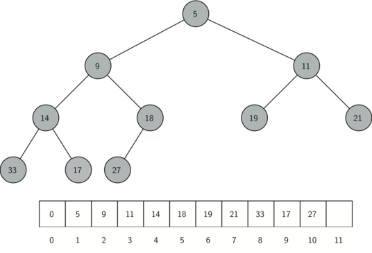
குவியல் செயல்பாடுகள் - Heap Operations
We will begin our implementation of a binary heap with the constructor. Since the entire binary heap can be represented by a single list, all the constructor will do is initialize the list and an attribute current_size to keep track of the current size of the heap. The code below shows the Python code for the constructor. You will notice that an empty binary heap has a single zero as the first element of items and that this zero is not used, but is there so that simple integer division can be used in later steps.
class BinaryHeap(object):
def __init__(self):
self.items = [0]
def __len__(self):
return len(self.items) - 1
The next method we will implement is insert. The easiest, and most efficient, way to add an item to a list is to simply append the item to the end of the list. The good news about appending is that it guarantees that we will maintain the complete tree property. The bad news about appending is that we will very likely violate the heap structure property. However, it is possible to write a method that will allow us to regain the heap structure property by comparing the newly added item with its parent. If the newly added item is less than its parent, then we can swap the item with its parent. The diagram below shows the series of swaps needed to percolate the newly added item up to its proper position in the tree.
Percolate the new node up to its proper position
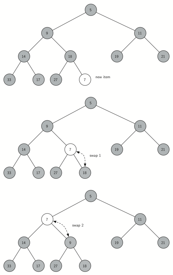
Notice that when we percolate an item up, we are restoring the heap property between the newly added item and the parent. We are also preserving the heap property for any siblings. Of course, if the newly added item is very small, we may still need to swap it up another level. In fact, we may need to keep swapping until we get to the top of the tree. The code below shows the percolate_up method, which percolates a new item as far up in the tree as it needs to go to maintain the heap property. Here is where our wasted element in items is important. Notice that we can compute the parent of any node by using simple integer division. The parent of the current node can be computed by dividing the index of the current node by 2.
def percolate_up(self):
i = len(self)
while i // 2 > 0:
if self.items[i] < self.items[i // 2]:
self.items[i // 2], self.items[i] = \
self.items[i], self.items[i // 2]
i = i // 2
We are now ready to write the insert method (see below). Most of the work in the insert method is really done by percolate_up. Once a new item is appended to the tree, percolate_up takes over and positions the new item properly.
def insert(self, k):
self.items.append(k)
self.percolate_up()
With the insert method properly defined, we can now look at the delete_min method. Since the heap property requires that the root of the tree be the smallest item in the tree, finding the minimum item is easy. The hard part of delete_min is restoring full compliance with the heap structure and heap order properties after the root has been removed. We can restore our heap in two steps. First, we will restore the root item by taking the last item in the list and moving it to the root position. Moving the last item maintains our heap structure property. However, we have probably destroyed the heap order property of our binary heap. Second, we will restore the heap order property by pushing the new root node down the tree to its proper position. The diagram shows the series of swaps needed to move the new root node to its proper position in the heap.
Percolating the root node down the tree
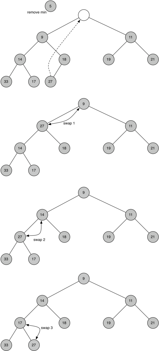
In order to maintain the heap order property, all we need to do is swap the root with its smallest child less than the root. After the initial swap, we may repeat the swapping process with a node and its children until the node is swapped into a position on the tree where it is already less than both children. The code for percolating a node down the tree is found in the percolate_down and min_child methods below.
def percolate_down(self, i):
while i * 2 <= len(self):
mc = self.min_child(i)
if self.items[i] > self.items[mc]:
self.items[i], self.items[mc] = self.items[mc], self.items[i]
i = mc
def min_child(self, i):
if i * 2 + 1 > len(self):
return i * 2
if self.items[i * 2] < self.items[i * 2 + 1]:
return i * 2
return i * 2 + 1
The code for the delete_min operation is below. Note that once again the hard work is handled by a helper function, in this case percolate_down.
def delete_min(self):
return_value = self.items[1]
self.items[1] = self.items[len(self)]
self.items.pop()
self.percolate_down(1)
return return_value
To finish our discussion of binary heaps, we will look at a method to build an entire heap from a list of keys. The first method you might think of may be like the following. Given a list of keys, you could easily build a heap by inserting each key one at a time. Since you are starting with a list of one item, the list is sorted and you could use binary search to find the right position to insert the next key at a cost of approximately O(log[n]) operations. However, remember that inserting an item in the middle of the list may require O(n) operations to shift the rest of the list over to make room for the new key. Therefore, to insert n keys into the heap would require a total of O(nlog[n]) operations. However, if we start with an entire list then we can build the whole heap in O(n) operations. The code below shows the code to build the entire heap.
def build_heap(self, alist):
i = len(alist) // 2
self.items = [0] + alist
while i > 0:
self.percolate_down(i)
i = i - 1
Building a heap from the list [9, 6, 5, 2, 3]
![Building a heap from the list [9, 6, 5, 2, 3]](https://lh7-us.googleusercontent.com/docs/AHkbwyJYv2AT8K0w9QtEB12Vu9LJwt7SqJiIeVmmW6Pub9a_OztQHVAoqPyQAfRxyZz7gNUgCyAS8o-h2YnCjz45_LTDbSp_alxt41-VZVj48udUNh47J6dk_PgnIeiYq1EE5sVNNOVaS3jqwdy8EMpiiDTYY6Utmyr_R0NXg1ePYgXD5-ntPaIh8prtEayYTV5tHJNU)
Above we see the swaps that the build_heap method makes as it moves the nodes in an initial tree of [9, 6, 5, 2, 3] into their proper positions. Although we start out in the middle of the tree and work our way back toward the root, the percolate_down method ensures that the largest child is always moved down the tree. Because the heap is a complete binary tree, any nodes past the halfway point will be leaves and therefore have no children. Notice that when i==1, we are percolating down from the root of the tree, so this may require multiple swaps. As you can see in the rightmost two trees of above, first the 9 is moved out of the root position, but after 9 is moved down one level in the tree, percolate_down ensures that we check the next set of children farther down in the tree to ensure that it is pushed as low as it can go. In this case it results in a second swap with 3. Now that 9 has been moved to the lowest level of the tree, no further swapping can be done. It is useful to compare the list representation of this series of swaps as shown in above with the tree representation.
i = 2 [0, 9, 5, 6, 2, 3]
i = 1 [0, 9, 2, 6, 5, 3]
i = 0 [0, 2, 3, 6, 5, 9]
The assertion that we can build the heap in O(n) may seem a bit mysterious at first, and a proof is beyond the scope of this book. However, the key to understanding that you can build the heap in O(n) is to remember that the log[n] factor is derived from the height of the tree. For most of the work in build_heap, the tree is shorter than log[n].
8.6 இருகிளை தேடல்மரம் - Binary Search Trees
தொர்புரு அணி சுருக்க தரவு வகையைச் செயல்படுத்த இரண்டு வெவ்வேறு வழிகளைப் பார்த்தோம் - அவை பட்டியலில் இரும நிலைத் தேடல் மற்றும் எண்ணிம அடைவு அட்டவணைகள் ஆகும் . இந்த பிரிவில் நாம் இருபடி மரத்தை கருத்தில் கொள்வோம், இது திறமையான தேடலில் கவனம் செலுத்தும் தொர்புரு அணிகளின் மற்றொரு பொதுவான செயலாக்கத்தின் அடிப்படையாகும்.
செயல்படுத்துவதைப் பார்ப்பதற்கு முன், ADT வரைபடம் வழங்கிய இடைமுகத்தை மதிப்பாய்வு செய்வோம். இந்த இடைமுகம் பைதான் தொடர்புறு அணியை ஒத்திருப்பதைக் கவனிக்கவும்.
- Map() புதிய, வெற்று தொர்புரு அணியை உருவாக்கவும்.
- put(key, val) தொர்புரு அணியில் புதிய சாவி-மதிப்பு ஜோடியைச் சேர்க்கவும்.ஏற்கனவே வரைபடத்தில் உள்ள சாவி என்றால் பழைய மதிப்பை புதிய மதிப்புடன் மாற்றவும்.
- get(key) ஒரு சாவி கொடுக்கப்பட்டால், தொர்புரு அணியில் சேமிக்கப்பட்ட மதிப்பைத் திருப்பி அனுப்பவும் அல்லது இல்லையெனில் இல்லை.
- del - del map[key] என்ற அறிக்கையைப் பயன்படுத்தி தொர்புரு அணியிலிருந்து சாவி-மதிப்பு ஜோடியை நீக்கவும்
- len() வரைபடத்தில் சேமிக்கப்பட்டுள்ள சாவி - மதிப்பு ஜோடிகளின் எண்ணிக்கையை வழங்கவும்.
- in கொடுக்கப்பட்ட சாவி தொர்புரு அணியில் உள்ளது என்றால் key in map அறிக்கைக்கு True என்பதைத் தரவும்.
செயற்படுத்தல் - Implementation
ஒரு இரு கிளைத் தேடல் மரம் குறைவாக உள்ள சாவிகளைச் சார்ந்துள்ளது.பெற்றோர் இடது துணை மரத்தில் காணப்படுகின்றன, மேலும் சாவிகள் அதிகமாக இருக்கும்.பெற்றோர் வலது துணை மரத்தில் காணப்படுகின்றனர். இதை நாம் BST property என்று அழைப்போம்.மேலே விவரிக்கப்பட்டுள்ளபடி `map ' இடைமுகத்தை செயல்படுத்தும்போது, BST property செயல்படுத்த வழிகாட்டும். கீழே உள்ள வரைபடம் இரு கிளைத் தேடல் மரத்தின் இந்தப் பண்புகளை விளக்குகிறது,மற்றும் தொடர்புடைய மதிப்புகள் இல்லாமல் சாவிகளைக் காட்டுகின்றது. பெற்றோர் மற்றும் குழந்தைகள் ஒவ்வொருவோருக்கும் மதிப்புள்ளது என்பதைக் கவனியுங்கள் இடது துணை மரத்திலுள்ள உள்ள அனைத்து சாவிகளையும் விட குறைவாக வேரில் சாவிகள் உள்ளன வலது துணை மரத்திலுள்ள உள்ள அனைத்து சாவிகளும் வேரிலுள்ளவற்றைவிடப் பெரியவை.
A simple binary search tree
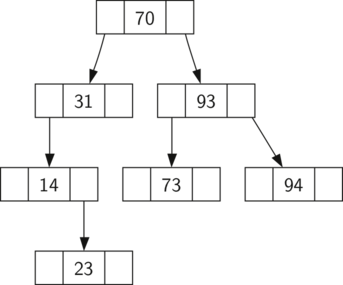
இருகிளைத் தேடல் மரம் என்றால் என்ன என்று இப்போது உங்களுக்குத் தெரியும், இருகிளைத் தேடல் மரம் எவ்வாறு உருவாக்கப்படுகிறது என்பதைப் பார்ப்போம். மேலே உள்ள தேடல் மரம் பின்வரும் சாவிகளை வரிசையாகச் செருகிய பின் இருக்கும் முனைகளைக் குறிக்கிறது: 70, 31, 93, 94, 14, 23, 73. 70 முதல் மரத்தில் செருகப்பட்ட சாவி என்பதால், அது வேர். அடுத்து, 31 என்பது 70க்குக் குறைவானது, எனவே அது 70 இன் இடது குழந்தையாகிறது. அடுத்து, 93 என்பது 70 ஐ விட பெரியது, எனவே அது 70 இன் வலது குழந்தையாகிறது. இப்போது மரத்தின் இரண்டு நிலைகள் நிரப்பப்பட்டுள்ளன, எனவே அடுத்த சாவிக்கு செல்கிறது. 31 அல்லது 93 இன் இடது அல்லது வலது குழந்தையாக இருக்க வேண்டும். 94 ஆனது 70 மற்றும் 93 ஐ விட பெரியதாக இருப்பதால், அது 93 இன் வலது குழந்தையாக மாறும். அதே போல் 14 ஆனது 70 மற்றும் 31 க்கு குறைவாக உள்ளது, எனவே அது 31 இன் இடது குழந்தையாகிறது. 23 ஆனது 31 க்கும் குறைவானது, எனவே இது 31 இன் இடது துணை மரத்தில் இருக்க வேண்டும். இருப்பினும், இது 14 ஐ விட அதிகமாக உள்ளது, எனவே அது 14 இன் வலது குழந்தையாகிறது.
இருகிளைத் தேடல் மரத்தை செயல்படுத்த, முனைகள் மற்றும் குறிப்புகள் அணுகுமுறையைப் பயன்படுத்துவோம். இந்த அத்தியாயத்தில் வேறு இடத்தில் உள்ளது போல் dict s ஐப் பயன்படுத்தி மரத்தை செயல்படுத்துவது பைத்தானில் சாத்தியம் என்றாலும், அவ்வாறு செய்வது நாம் செயல்படுத்தும் துணை அமைப்பு நம்மிடம் இருப்பதை முன்னறிவிக்கிறது!
எங்கள் செயல்படுத்தல் இரண்டு வகுப்புகளைப் பயன்படுத்தும்: TreeNode மரத்தையே கட்டமைக்கவும் கையாளவும் கீழ் நிலை தர்க்கத்தை அமைக்கவும், BinarySearchTreeஆனது வேர் முனை பற்றிய குறிப்பை வைத்திருக்கவும் மற்றும் பயனருக்கு தொர்புரு அணி போன்ற இடைமுகத்தை வழங்கும்.
The TreeNode class provides many helper functions that make the work done in the BinarySearchTree class methods much easier. The constructor for a TreeNode, along with these helper functions, is shown below. As you can see, many of these helper functions help to classify a node according to its own position as a child, (left or right) and the kind of children the node has. The TreeNode class will also explicitly keep track of the parent as an attribute of each node. You will see why this is important when we discuss the implementation for the del operator.
One of the more interesting methods of TreeNode provides an interface to simply iterate over all the keys in the tree in order. You already know how to traverse a binary tree in order, using the inorder traversal algorithm. However, because we want our iterator to operate lazily, in this case we use the yield keyword to define our __iter__ method as a Python generator. Pay close attention to the __iter__ implementation as at first glance you might think that the code is not recursive: in fact, because __iter__ overrides the for x in operation for iteration, it really is recursive!
Our full implementation of TreeNode is provided below. It includes three further methods find_successor, find_min and splice_out which you can ignore for now as we will return to them later when discussing deletion.
class TreeNode(object):
def __init__(self, key, val, left=None, right=None, parent=None):
self.key = key
self.val = val
self.left = left
self.right = right
self.parent = parent
def is_left_child(self):
return self.parent and self.parent.left == self
def is_right_child(self):
return self.parent and self.parent.right == self
def is_leaf(self):
return not (self.right or self.left)
def has_any_children(self):
return self.right or self.left
def has_both_children(self):
return self.right and self.left
def has_one_child(self):
return self.has_any_children() and not self.has_both_children()
def replace_node_data(self, key, val, left, right):
self.key = key
self.val = val
self.left = left
self.right = right
if self.left:
self.left.parent = self
if self.right:
self.right.parent = self
def __iter__(self):
if self is None:
return
if self.left:
# `in` calls `__iter__` so is recursive
for elem in self.left:
yield elem
yield self.key
if self.right:
# recurse again
for elem in self.right:
yield elem
def find_successor(self):
if self.right:
return self.right.find_min()
if self.parent is None:
return None
if self.is_left_child():
return self.parent
self.parent.right = None
successor = self.parent.find_successor()
self.parent.right = self
return successor
def find_min(self):
current = self
while current.left:
current = current.left
return current
def splice_out(self):
if self.is_leaf():
if self.is_left_child():
self.parent.left = None
else:
self.parent.right = None
else:
promoted_node = self.left or self.right
if self.is_left_child():
self.parent.left = promoted_node
else:
self.parent.right = promoted_node
promoted_node.parent = self.parent
Now that we have our TreeNode class we can begin to write BinarySearchTree itself. Recall that the core functionality of this class will be to enable puting to and geting from the tree, so we begin our implementation with the put functionality.
In order to enable the tree[1] = 'foo' style assignment interface for our BinarySearchTree instances, we override the __setitem__ magic method. In this method we first check to see if the tree already has a root. If there is not a root then we create a new TreeNode and set it as the root of the tree. If a root node is already in place then put calls the private, recursive, helper function _put to search the tree according to the following algorithm:
- Starting at the root of the tree, search the binary tree comparing the new key to the key in the current node. If the new key is less than the current node, search the left subtree. If the new key is greater than the current node, search the right subtree.
- When there is no left (or right) child to search, we have found the position in the tree where the new node should be installed.
- To add a node to the tree, create a new TreeNode object and insert the object at the point discovered in the previous step.
The code below shows the Python code for inserting a new node in the tree. The _put function is written recursively following the steps outlined above. Notice that when a new child is inserted into the tree, the node is passed to the new tree as the parent.
One important problem with our implementation of insert is that duplicate keys are not handled properly. As our tree is implemented a duplicate key will create a new node with the same key value in the right subtree of the node having the original key. The result of this is that the node with the new key will never be found during a search. A better way to handle the insertion of a duplicate key is for the value associated with the new key to replace the old value. We leave fixing this bug as an exercise for you.
class BinarySearchTree(object):
TreeNodeClass = TreeNode
def __init__(self):
self.root = None
self.size = 0
def __len__(self):
return self.size
def __iter__(self):
return self.root.__iter__()
def __setitem__(self, key, val):
if self.root:
self._put(key, val, self.root)
else:
self.root = self.TreeNodeClass(key, val)
self.size = self.size + 1
def _put(self, key, val, node):
if key < node.key:
if node.left:
self._put(key, val, node.left)
else:
node.left = self.TreeNodeClass(key, val, parent=node)
else:
if node.right:
self._put(key, val, node.right)
else:
node.right = self.TreeNodeClass(key, val, parent=node)
The diagram below illustrates the process for inserting a new node into a binary search tree. The lightly shaded nodes indicate the nodes that were visited during the insertion process.
Inserting a node with key = 19
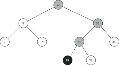
Once the tree is constructed, the next task is to implement the retrieval of a value for a given key. The get functionality is even easier than the put functionality because we simply search the tree recursively until we get to a non-matching leaf node or find a matching key. When a matching key is found, the value stored in the val of the node is returned.
Again, inorder to enable a tree[1] retrieval interface, we overload one of Python’s magic methods—in this case __getitem__. Just like with __setitem__, the primary purpose of this method is to handle presence and absence of a root node, and delegates the core get functionality to _get.
The search code in the _get method uses the same logic for choosing the left or right child as the _put method. Notice that the _get method returns a TreeNode to __getitem__, this allows _get to be used as a flexible helper method for other BinarySearchTree methods that may need to make use of other data from the TreeNode besides the val.
def __getitem__(self, key):
if self.root:
result = self._get(key, self.root)
if result:
return result.val
raise KeyError
def _get(self, key, node):
if not node:
return None
if node.key == key:
return node
if key < node.key:
return self._get(key, node.left)
return self._get(key, node.right)
Using _get, we can implement the in operation by writing a __contains__ method for the BinarySearchTree. The __contains__ method will simply call _get and return True if _get returns a value, or False if it returns None. The code for __contains__ is shown below.
def __contains__(self, key):
return bool(self._get(key, self.root))
Finally, we turn our attention to the most challenging method in the binary search tree: the deletion of a key. The first task is to find the node to delete by searching the tree. If the tree has more than one node we search using the _get method to find the TreeNode that needs to be removed. If the tree only has a single node, that means we are removing the root of the tree, but we still must check to make sure the key of the root matches the key that is to be deleted. In either case if the key is not found the del operator raises an error.
def delete(self, key):
if self.size > 1:
node_to_remove = self._get(key, self.root)
if node_to_remove:
self.remove(node_to_remove)
self.size = self.size - 1
return
elif self.size == 1 and self.root.key == key:
self.root = None
self.size = self.size - 1
return
raise KeyError('Error, key not in tree')
def __delitem__(self, key):
self.delete(key)
Once we’ve found the node containing the key we want to delete, there are three cases that we must consider:
- The node to be deleted has no children
- The node to be deleted has only one child
- The node to be deleted has two children
The first case is straightforward. If the current node has no children all we need to do is delete the node and remove the reference to this node in the parent. The code for this case is shown below.
def remove(self, node):
if node.is_leaf() and node.parent is not None:
if node == node.parent.left:
node.parent.left = None
else:
node.parent.right = None
Deleting Node 16, a node without children
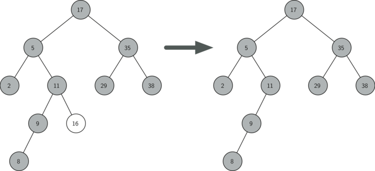
The second case is only slightly more complicated (see below). If a node has only a single child, then we can simply promote the child to take the place of its parent. The code for this case is shown in the next code sample. As you look at this code you will see that there are six cases to consider. Since the cases are symmetric with respect to either having a left or right child we will just discuss the case where the current node has a left child. The decision proceeds as follows:
- If the current node is a left child then we only need to update the parent reference of the left child to point to the parent of the current node, and then update the left child reference of the parent to point to the current node’s left child.
- If the current node is a right child then we only need to update the parent reference of the right child to point to the parent of the current node, and then update the right child reference of the parent to point to the current node’s right child.
- If the current node has no parent, it must be the root. In this case we will just replace the key, val, left, and right data by calling the replace_node_data method on the root.
Code for this decision process may look like:
elif node.has_one_child():
promoted_node = node.left or node.right
if node.is_left_child():
promoted_node.parent = node.parent
node.parent.left = promoted_node
elif node.is_right_child():
promoted_node.parent = node.parent
node.parent.right = promoted_node
else:
node.replace_node_data(
promoted_node.key,
promoted_node.val,
promoted_node.left,
promoted_node.right
)
Deleting node 25, a node that has a single child
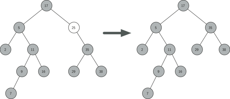
The third case is the most difficult case to handle (see below). If a node has two children, then it is unlikely that we can simply promote one of them to take the node’s place. We can, however, search the tree for a node that can be used to replace the one scheduled for deletion. What we need is a node that will preserve the binary search tree relationships for both of the existing left and right subtrees. The node that will do this is the node that has the next-largest key in the tree. We call this node the successor, and we will look at a way to find the successor shortly. The successor is guaranteed to have no more than one child, so we know how to remove it using the two cases for deletion that we have already implemented. Once the successor has been removed, we simply put it in the tree in place of the node to be deleted.
Deleting node 5, a node with two children
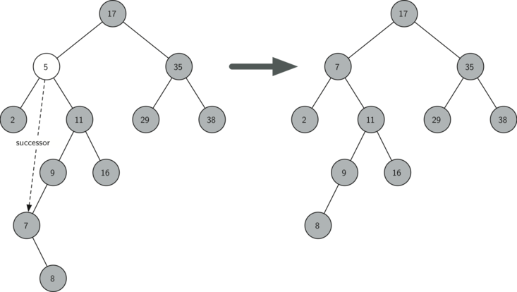
The code to handle the third case is shown below. Notice that we make use of the helper methods find_successor and find_min to find the successor. To remove the successor, we make use of the method splice_out. The reason we use splice_out is that it goes directly to the node we want to splice out and makes the right changes. We could call delete recursively, but then we would waste time re-searching for the key node.
else: # has both children
successor = node.find_successor()
if successor:
successor.splice_out()
node.key = successor.key
node.val = successor.val
The code to find the successor is shown above and as you can see is a method of the TreeNode class. This code makes use of the same properties of binary search trees that cause an inorder traversal to print out the nodes in the tree from smallest to largest. There are three cases to consider when looking for the successor:
- If the node has a right child, then the successor is the smallest key in the right subtree.
- If the node has no right child and is the left child of its parent, then the parent is the successor.
- If the node is the right child of its parent, and itself has no right child, then the successor to this node is the successor of its parent, excluding this node.
The first condition is the only one that matters for us when deleting a node from a binary search tree.
The find_min method is called to find the minimum key in a subtree. You should convince yourself that the minimum valued key in any binary search tree is the leftmost child of the tree. Therefore the find_min method simply follows the left references in each node of the subtree until it reaches a node that does not have a left child.
திறனாய்வு - Analysis
இருகிளைத் தேடல் மரத்தின் செயலாக்கம் முடிந்ததும்,நாங்கள் செயல்படுத்திய முறைகளின் விரைவான திறனாய்வை நாங்கள் செய்வோம். முதலில் put முறை நாங்கள் பார்ப்போம் . அதன் செயல்திறனில் கட்டுப்படுத்தும் காரணி இருகிளை மரத்தின் உயரம் ஆகும்.ஒரு மரத்தின் வேர் மற்றும் ஆழமான இலை முனை இடையே உள்ள விளிம்புகளின் எண்ணிக்கை உயரம் என்பதை என்பதை நினைவில் கொள்க.. நாம் தேடும் போது உயரம் கட்டுப்படுத்தும் காரணியாகும். ஏனென்றால் மரத்தில் ஒரு முனையைச் செருகுவதற்கு பொருத்தமான இடம், நமக்குத் தேவைப்படும் மரத்தின் ஒவ்வொரு மட்டத்திலும் அதிகபட்சம் ஒரு ஒப்பீடு செய்ய வேண்டும்.
இருகிளை மரத்தின் உயரம் என்னவாக இருக்கும்? இதற்கான பதில் மரத்தில் சாவிகள் எவ்வாறு சேர்க்கப்படுகின்றன என்பதைப் பொறுத்தது. சாவிகள் இருந்தால் சீரற்ற வரிசையில் சேர்த்தால், மரத்தின் உயரம் சுற்றி இருக்கும் $$\log_2{n}$$ இங்கு $$n$$ என்பது மரத்தில் உள்ள முனைகளின் எண்ணிக்கை. இது ஏனெனில் சாவிகள் தோராயமாக விநியோகிக்கப்பட்டதாலாகும் , அவற்றில் பாதி வேரை விட குறைவாகவும் ,பாதி வேரை விட அதிகமாகவும் இருக்கும். அதை நினைவில் கொள்க ஒரு இருகிளை மரத்தில் வேரில் ஒரு முனையும், அடுத்த நிலையில் இரண்டு முனைகளும் உள்ளன மற்றும் நிலையில் அடுத்த நான்கு முனைகளும் உள்ளன. எந்த குறிப்பிட்ட மட்டத்திலும் உள்ள முனைகளின் எண்ணிக்கை 2d ஆகும் d என்பது மட்டத்தின் ஆழம். முனைகளின் மொத்த எண்ணிக்கை ஒரு முழுமையான சமநிலையான இருகிளை மரத்தில் 2h+1-1, ஆகும் h என்பது மரத்தின் உயரத்தைக் குறிக்கும்.
ஒரு முழுமையான சீரான மரமானது, வலது துணை மரத்தில் உள்ள அதே எண்ணிக்கையிலான முனைகளைக் கொண்டது. சமநிலையான இருகிளை மரத்தில், put இன் மோசமான செயல்திறன் O(log2[n]), இங்கு n என்பது மரத்தில் உள்ள முனைகளின் எண்ணிக்கை. முந்தைய பத்தியில் உள்ள கணக்கீட்டிற்கு இது நேர்மாறான தொடர்பு என்பதை கவனியுங்கள். எனவே log2[n] மரத்தின் உயரத்தைக் கொடுக்கிறது, மேலும் புதிய முனையைச் செருகுவதற்கான சரியான இடத்தைத் தேடும் போது செய்ய வேண்டிய அதிகபட்ச ஒப்பீடுகளின் எண்ணிக்கையைக் குறிக்கிறது.
துரதிருஷ்டவசமாக வரிசைப்படுத்தப்பட்ட வரிசையில் சாவிகளை செருகுவதன் மூலம் n உயரம் கொண்ட ஒரு தேடல் மரத்தை உருவாக்க முடியும்! அத்தகைய மரத்தின் உதாரணம் கீழே காட்டப்பட்டுள்ளது. இந்த வழக்கில் put முறையின் செயல்திறன் O(n) ஆகும்.
A skewed binary search tree would give poor performance
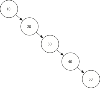
put முறையின் செயல்திறன் மரத்தின் உயரத்தால் வரையறுக்கப்பட்டுள்ளது என்பதை இப்போது நீங்கள் புரிந்துகொள்கிறீர்கள், மற்ற முறைகளான get, in, , மற்றும் delஆகியவையும் குறைவாகவே இருக்கும் என்று நீங்கள் யூகிக்க முடியும். மரத்தைத் தேடுவதால், சாவியைக் கண்டுபிடிக்க, மிக மோசமான நிலையில், மரத்தின் அடிப்பகுதி வரை தேடியும் எந்தச் சாவியும் கிடைக்கவில்லை. முதல் பார்வையில் del மிகவும் சிக்கலானதாகத் தோன்றலாம், ஏனெனில் நீக்குதல் செயல்பாடு முடிவடைவதற்கு முன் வாரிசைத் தேட வேண்டியிருக்கும். ஆனால் வாரிசைக் கண்டுபிடிப்பதற்கான மோசமான சூழ்நிலை மரத்தின் உயரம் மட்டுமே என்பதை நினைவில் கொள்ளுங்கள், அதாவது நீங்கள் வேலையை இரட்டிப்பாக்குவீர்கள். இரட்டிப்பு ஒரு நிலையான காரணி என்பதால் அது மோசமான நிலையில் மாறாது.
8.7 AVL மரம் தரவமைப்பு - AVL Trees
முந்தைய பகுதியில் இரும நிலைத் தேடல் மரத்தை உருவாக்குவதைப் பார்த்தோம். நாம் அறிந்தது போல், மரம் சமநிலையற்றதாக இருக்கும்போது, பெறுதல் மற்றும் போடுதல் போன்ற செயல்பாடுகளுக்கு இரும நிலைத் தேடல் மரத்தின் செயல்திறன் O(n) க்கு குறையும். இந்த பிரிவில், ஒரு சிறப்பு வகையான இரும நிலைத் தேடல் மரத்தைப் பார்ப்போம், மரம் எல்லா நேரங்களிலும் சமநிலையில் இருப்பதை தானாகவே உறுதிசெய்கிறது. இந்த மரம் அதன் கண்டுபிடிப்பாளர்களின் பெயரால் AVL மரம் என்று அழைக்கப்படுகிறது: ஜி.எம். அடெல்சன்-வெல்ஸ்கி மற்றும் ஈ.எம். லாண்டிஸ். சுய-சமநிலை இரும நிலைத் தேடல் மரங்களுக்கு உதாரணமாக AVL மரங்களில் கவனம் செலுத்த முடிவு செய்துள்ளோம், ஆனால் பிரபலமான red-black tree போன்ற பல உள்ளன.
AVL மரம் ஒரு வழக்கமான இரும நிலைத் தேடல் மரத்தைப் போலவே தொடர்புறு அணி சுருக்க தரவு வகையைச் செயல்படுத்துகிறது, மரம் எவ்வாறு செயல்படுகிறது என்பதில் மட்டுமே வேறுபாடு உள்ளது. எங்கள் AVL மரத்தை செயல்படுத்த, மரத்தில் உள்ள ஒவ்வொரு முனைக்கும் சமநிலை காரணியை நாம் கண்காணிக்க வேண்டும். ஒவ்வொரு முனைக்கும் இடது மற்றும் வலது துணை மரங்களின் உயரங்களைப் பார்த்து இதைச் செய்கிறோம். இன்னும் முறையாக, ஒரு முனைக்கான சமநிலை காரணியை இடது துணை மரத்தின் உயரத்திற்கும் வலது துணை மரத்தின் உயரத்திற்கும் உள்ள வித்தியாசமாக வரையறுக்கிறோம்.
balanceFactor = height(leftSubTree) − height(rightSubTree)
மேலே கொடுக்கப்பட்ட சமநிலை காரணிக்கான வரையறையைப் பயன்படுத்தி,சமநிலை காரணி பூஜ்ஜியத்தை விட அதிகமாக இருந்தால் துணைமரம் இடதுபுறம் கனமாக இருக்கும்.சமநிலை காரணி பூஜ்ஜியத்தை விட குறைவாக இருந்தால், துணை மரம் வலதுபுறம் கனமாக இருக்கும். சமநிலை காரணி பூஜ்ஜியமாக இருந்தால், மரம் சரியாக சமநிலையில் உள்ளது. என்று எங்களால் கூறமுடியும்.AVL மரத்தை செயல்படுத்துவதன் நோக்கங்கள் மற்றும் அதன் பலனைப் பெறுதல் ஒரு சமநிலை மரம் சமநிலையில் இருந்தால் ஒரு மரத்தை சமநிலையில் இருக்கும் என்று வரையறுப்போம் சமநிலைக் காரணி -1, 0 அல்லது 1 ஆகும். ஒரு மரம் ஒன்றில் ஒரு முனையின் சமநிலைக்கு காரணி வரம்பிற்கு வெளியே இருந்தால் அந்த மரத்தை மீண்டும் சமநிலைக்கு கொண்டு வர சில படிமுறைகளை நாம் கொண்டிருக்க வேண்டும்.கீழே உள்ள படம் வலதுபுறம் கனமான, சமநிலையற்ற மரம் மற்றும் ஒவ்வொரு முனைக்குமான சமநிலைக்கு காரணிகளையும் காட்டுகின்றது.
An unbalanced right-heavy tree with balance factors
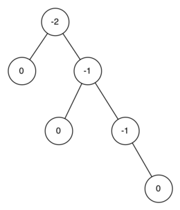
நாம் மேலும் தொடர்வதற்கு முன், இந்த புதிய சமநிலை காரணி தேவையை அமுல்படுத்துவதன் முடிவைப் பார்ப்போம். எங்கள் கூற்று என்னவென்றால், ஒரு மரத்தில் எப்போதும் சமநிலை காரணி -1, 0 அல்லது 1 ஆக இருப்பதை உறுதி செய்வதன் மூலம் முக்கிய செயல்பாடுகளின் சிறந்த பெரிய O செயல்திறனைப் பெறலாம். இந்த சமநிலை நிலை மோசமான மரத்தை எவ்வாறு மாற்றுகிறது என்பதைப் பற்றி சிந்திக்க ஆரம்பிக்கலாம். கருத்தில் கொள்ள இரண்டு சாத்தியக்கூறுகள் உள்ளன, ஒரு இடது கனமான மரம் மற்றும் ஒரு வலது கனமான மரம். 0, 1, 2 மற்றும் 3 உயரமுள்ள மரங்களை நாம் கருத்தில் கொண்டால், கீழே உள்ள வரைபடம் புதிய விதிகளின் கீழ் சாத்தியமான மிகவும் சமநிலையற்ற இடது-கனமான மரத்தை விளக்குகிறது.
Worst-case left-heavy AVL trees
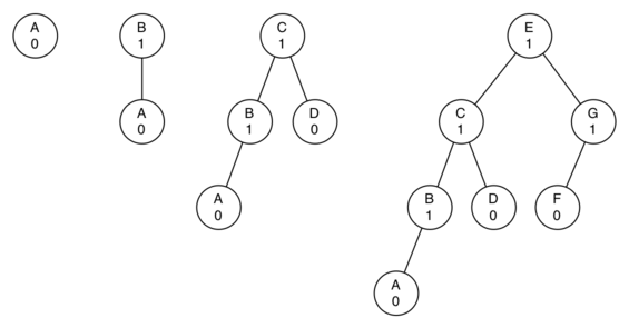
மரத்தில் உள்ள மொத்த முனைகளின் எண்ணிக்கையைப் பார்த்தால், உயரம் 0 இல் ஒரு மரம் உள்ளது அதில் 1 முனை உள்ளது, உயரம் 1 உள்ள மரத்திற்கு 1+1 = 2 முனைகள் உள்ளது, உயரம் 2 உள்ள மரத்திற்கு 1+1+2 = 4 மற்றும் உயரம் 3 இல் உள்ள மரத்திற்கு 1 + 2 + 4 = 7 முனைகள் உள்ளன. பொதுவாக நாம் பார்க்கும் முறை h (Nh) உயரமுள்ள மரத்தில் உள்ள முனைகளின் எண்ணிக்கை.
Nh=1+Nh−1+Nh−2
இந்த மறுநிகழ்வு உங்களுக்கு நன்கு தெரிந்திருக்கலாம், ஏனெனில் இது பிபினாச்சி வரிசைக்கு மிகவும் ஒத்திருக்கிறது. மரத்தில் உள்ள முனைகளின் எண்ணிக்கையைக் கொண்டு AVL மரத்தின் உயரத்திற்கான சூத்திரத்தைப் பெற இந்த உண்மையைப் பயன்படுத்தலாம். பிபினாச்சி வரிசைக்கு i_{th} பிபினாச்சி எண் கொடுக்கப்பட்டிருப்பதை நினைவுபடுத்தவும்:
F0=0
F1=1
Fi=Fi-1 + Fi−2 for all i ≥ 2 Fi = Fi-1 + Fi-2 ∀ i ≥ 2
An important mathematical result is that as the numbers of the Fibonacci sequence get larger and larger the ratio of Fi/Fi−1 becomes closer and closer to approximating the golden ratio Φ which is defined as Φ=(1+√5)/2. You can consult a math text if you want to see a derivation of the previous equation. We will simply use this equation to approximate Fi = Φi/√5. If we make use of this approximation we can rewrite the equation for Nh as:
Nh=Fh+2−1, h≥1
By replacing the Fibonacci reference with its golden ratio approximation we get:
Nh=Φh+2 /√5−1
If we rearrange the terms, and take the base 2 log of both sides and then solve for h we get the following derivation:
log[Nh+1]=(H+2)log[Φ]−½ log[5]
h=( log[Nh+1]−2 log[Φ] + ½log[5] ) /logΦ
h=1.44 log[Nh]
This derivation shows us that at any time the height of our AVL tree is equal to a constant(1.44) times the log of the number of nodes in the tree. This is great news for searching our AVL tree because it limits the search to O(logN).
செயல்படுத்தல் - Implementation
AVL மரத்தை சமநிலையில் வைத்திருப்பது ஒரு பெரிய செயல்திறன் முன்னேற்றமாக இருக்கும் என்பதை இப்போது நாங்கள் நிரூபித்துள்ளோம், மரத்தில் ஒரு புதிய சாவியை செருகுவதற்கான செயல்முறையை எவ்வாறு அதிகரிப்பது என்பதைப் பார்ப்போம். அனைத்து புதிய சாவிகளுக்கும் இலை முனைகளாக மரத்தில் செருகப்பட்டிருப்பதால், புதிய இலைக்கான இருப்பு காரணி பூஜ்ஜியம் என்பதை நாம் அறிவோம், இப்போது செருகப்பட்ட முனைக்கு புதிய தேவைகள் எதுவும் இல்லை. ஆனால் புதிய இலை சேர்க்கப்பட்டவுடன் அதன் பெற்றோரின் சமநிலை காரணியை நாம் புதுப்பிக்க வேண்டும். இந்த புதிய இலை பெற்றோரின் சமநிலை காரணியை எவ்வாறு பாதிக்கிறது என்பது இலை முனை இடது குழந்தையா அல்லது வலது குழந்தையா என்பதைப் பொறுத்தது. புதிய முனை சரியான குழந்தையாக இருந்தால், பெற்றோரின் சமநிலை காரணி ஒன்று குறைக்கப்படும். புதிய முனை இடது குழந்தையாக இருந்தால், பெற்றோரின் சமநிலை காரணி ஒன்று அதிகரிக்கும். இந்த உறவை புதிய முனையின் தாத்தா பாட்டிக்கும், மரத்தின் வேர் வரை ஒவ்வொரு மூதாதையருக்கும் மீண்டும் மீண்டும் பயன்படுத்தலாம். இது ஒரு சுழல்நிலை செயல்முறை என்பதால் சமநிலை காரணிகளைப் புதுப்பிப்பதற்கான இரண்டு அடிப்படை நிகழ்வுகளை ஆராய்வோம்:
- சுழற்சி அழைப்பு மரத்தின் வேரை அடைந்துள்ளது.
- பெற்றோரின் இருப்பு காரணி பூஜ்ஜியத்திற்கு சரிசெய்யப்பட்டது. ஒரு துணை மரமானது பூஜ்ஜியத்தின் சமநிலை காரணியைப் பெற்றவுடன், அதன் மூதாதையர் முனைகளின் சமநிலை மாறாது என்பதை நீங்கள் நம்பிக் கொள்ள வேண்டும்
எல்லா நேரங்களிலும் மரத்தை சமநிலையில் வைத்திருப்பதன் மூலம், get முறை O(log2[n]) நேரத்தில் இயங்குவதை உறுதிசெய்யலாம். ஆனால் கேள்வி என்னவென்றால், எங்கள் put முறைக்கு என்ன செலவு ? put முறை செயற்படுவதன் அடிப்படியில் செயற்பாடுகளை சிறியதாக பிரிக்கலாம்.ஒரு புதிய முனை இலையாகச் செருகப்பட்டிருப்பதால், அனைத்து பெற்றோரின் சமநிலை காரணிகளையும் புதுப்பிக்க அதிகபட்சமாக log2[n] செயல்பாடுகள் தேவைப்படும்,அது மரத்தின் ஒவ்வொரு நிலைக்கும் ஒன்று ஆகும். ஒரு துணை மரம் சமநிலையில் இல்லை எனில், மரத்தை மீண்டும் சமநிலைக்கு கொண்டு வர அதிகபட்சம் இரண்டு சுழற்சிகள் தேவை. ஆனால், ஒவ்வொரு சுழற்சியும் O(1) நேரத்தில் வேலை செய்கிறது, எனவே நமது get செயல்பாடு கூட O(log2[n]) ஆகவே இருக்கும்.
இந்த கட்டத்தில் நாங்கள் ஒரு செயல்பாட்டு AVL-Tree ஐ செயல்படுத்தியுள்ளோம், நீங்கள் ஒரு முனையை நீக்கும் திறன் தேவைப்படாவிட்டால். உங்களுக்கான ஒரு பயிற்சியாக முனையை நீக்குவதையும், அதைத் தொடர்ந்து புதுப்பித்து மறு சமநிலைப்படுத்துவதையும் விட்டுவிடுகிறோம்.
கடந்த சில பிரிவுகளில் வரைபட சுருக்க தரவு வகையைச் செயல்படுத்தப் பயன்படுத்தக்கூடிய பல தரவு கட்டமைப்புகளைப் பார்த்தோம். ஒரு பட்டியலில் ஒரு இப்படி தேடல், ஒரு தொர்புறு அணி அட்டவணை, ஒரு இரும நிலைத் தேடல் மரம் மற்றும் ஒரு சமநிலை இரும நிலைத் தேடல் மரம். இந்தப் பிரிவை முடிக்க, ADT வரைபடத்தால் வரையறுக்கப்பட்ட முக்கிய செயல்பாடுகளுக்கான ஒவ்வொரு தரவு கட்டமைப்பின் செயல்திறனையும் சுருக்கமாகக் கூறுவோம்.
from binary_search_tree import BinarySearchTree, TreeNode
class AVLTreeNode(TreeNode):
def __init__(self, *args, **kwargs):
super(AVLTreeNode, self).__init__(*args, **kwargs)
self.balance_factor = 0
class AVLTree(BinarySearchTree):
TreeNodeClass = AVLTreeNode
def _put(self, key, val, node):
if key < node.key:
if node.left:
self._put(key, val, node.left)
else:
node.left = self.TreeNodeClass(key, val, parent=node)
self.update_balance(node.left)
else:
if node.right:
self._put(key, val, node.right)
else:
node.right = self.TreeNodeClass(key, val, parent=node)
self.update_balance(node.right)
def update_balance(self, node):
if node.balance_factor > 1 or node.balance_factor < -1:
self.rebalance(node)
return
if node.parent is not None:
if node.is_left_child():
node.parent.balance_factor += 1
elif node.is_right_child():
node.parent.balance_factor -= 1
if node.parent.balance_factor != 0:
self.update_balance(node.parent)
The new update_balance method is where most of the work is done. This implements the recursive procedure we just described. The update_balance method first checks to see if the current node is out of balance enough to require rebalancing. If that is the case then the rebalancing is done and no further updating to parents is required. If the current node does not require rebalancing then the balance factor of the parent is adjusted. If the balance factor of the parent is non-zero then the algorithm continues to work its way up the tree toward the root by recursively calling update_balance on the parent.
When a rebalancing of the tree is necessary, how do we do it? Efficient rebalancing is the key to making the AVL Tree work well without sacrificing performance. In order to bring an AVL Tree back into balance we will perform one or more rotations on the tree.
To understand what a rotation is let us look at a very simple example. Consider the tree in the left half of the illustration below. This tree is out of balance with a balance factor of -2. To bring this tree into balance we will use a left rotation around the subtree rooted at node A.
Transforming an unbalanced tree using a left rotation
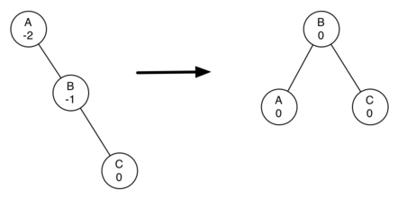
To perform a left rotation we essentially do the following:
- Promote the right child (B) to be the root of the subtree.
- Move the old root (A) to be the left child of the new root.
- If new root (B) already had a left child then make it the right child of the new left child (A). Note: Since the new root (B) was the right child of A the right child of A is guaranteed to be empty at this point. This allows us to add a new node as the right child without any further consideration.
While this procedure is fairly easy in concept, the details of the code are a bit tricky since we need to move things around in just the right order so that all properties of a Binary Search Tree are preserved. Furthermore we need to make sure to update all of the parent pointers appropriately.
Let’s look at a slightly more complicated tree to illustrate the right rotation. The left side of the illustration below shows a tree that is left-heavy and with a balance factor of 2 at the root. To perform a right rotation we essentially do the following:
- Promote the left child (C) to be the root of the subtree.
- Move the old root (E) to be the right child of the new root.
- If the new root(C) already had a right child (D) then make it the left child of the new right child (E). Note: Since the new root (C) was the left child of E, the left child of E is guaranteed to be empty at this point. This allows us to add a new node as the left child without any further consideration.
Transforming an unbalanced tree using a right rotation
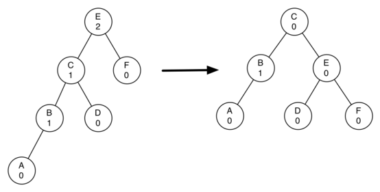
Now that you have seen the rotations and have the basic idea of how a rotation works let us look at the code below for both the left rotations. First we create a temporary variable to keep track of the new root of the subtree. As we said before the new root is the right child of the previous root. Now that a reference to the right child has been stored in this temporary variable we replace the right child of the old root with the left child of the new.
The next step is to adjust the parent pointers of the two nodes. If new_root has a left child then the new parent of the left child becomes the old root. The parent of the new root is set to the parent of the old root. If the old root was the root of the entire tree then we must set the root of the tree to point to this new root. Otherwise, if the old root is a left child then we change the parent of the left child to point to the new root; otherwise we change the parent of the right child to point to the new root. Finally we set the parent of the old root to be the new root. This is a lot of complicated bookkeeping, so we encourage you to trace through this function while looking at the diagram above.
def rotate_left(self, rotation_root):
new_root = rotation_root.right
rotation_root.right = new_root.left
if new_root.left is not None:
new_root.left.parent = rotation_root
new_root.parent = rotation_root.parent
if not rotation_root.parent:
self.root = new_root
else:
if rotation_root.is_left_child():
rotation_root.parent.left = new_root
else:
rotation_root.parent.right = new_root
new_root.left = rotation_root
rotation_root.parent = new_root
rotation_root.balance_factor = \
rotation_root.balance_factor + 1 - min(new_root.balance_factor, 0)
new_root.balance_factor = \
new_root.balance_factor + 1 + max(rotation_root.balance_factor, 0)
def rotate_right(self, rotation_root):
new_root = rotation_root.left
rotation_root.left = new_root.right
if new_root.right is not None:
new_root.right.parent = rotation_root
new_root.parent = rotation_root.parent
if not rotation_root.parent:
self.root = new_root
else:
if rotation_root.is_right_child():
rotation_root.parent.right = new_root
else:
rotation_root.parent.left = new_root
new_root.right = rotation_root
rotation_root.parent = new_root
rotation_root.balance_factor = \
rotation_root.balance_factor + 1 - min(new_root.balance_factor, 0)
new_root.balance_factor = \
new_root.balance_factor + 1 + max(rotation_root.balance_factor, 0)
The last two lines require some explanation. In these lines we update the balance factors of the old and the new root. Since all the other moves are moving entire subtrees around the balance factors of all other nodes are unaffected by the rotation. But how can we update the balance factors without completely recalculating the heights of the new subtrees? The following derivation should convince you that these lines are correct.
A left rotation
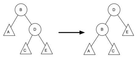
Above we see a left rotation. B and D are the pivotal nodes and A, C, E are their subtrees. Let hx denote the height of a particular subtree rooted at node x. By definition we know the following:
newBal(B)=hA−hC
oldBal(B)=hA−hD
But we know that the old height of D can also be given by 1+max(hC,hE)1 + max(h_C,h_E)1+max(hC,hE), that is, the height of D is one more than the maximum height of its two children. Remember that hch_chc and hE hav not changed. So, let us substitute that in to the second equation, which gives us
oldBal(B)=hA−(1+max(hC,hE))
and then subtract the two equations. The following steps do the subtraction and use some algebra to simplify the equation for newBal(B)
newBal(B)−oldBal(B)=hA−hC−(hA−(1+max(hC,hE)))
newBal(B)−oldBal(B)=hA−hC−hA+(1+max(hC,hE))
newBal(B)−oldBal(B)=1+max(hC,hE)−hC
Next we will move oldBal(B) to the right hand side of the equation and make use of the fact that max(a,b)−c=max(a−c,b−c):
newBal(B)−oldBal(B)=1+max(0,hE−hC)
But, hE−hC is the same as −oldBal(D). So we can use another identity that says max(−a,−b)=−min(a,b). So we can finish our derivation of newBal(B)newBal(B)newBal(B) with the following steps:
newBal(B)=oldBal(B)+1+max(0,−oldBal(D))
newBal(B)=oldBal(B)+1−min(0,oldBal(D))
Now we have all of the parts in terms that we readily know. If we remember that B is rotation_root and D is new_root then we can see this corresponds exactly to the statement on the penulitmate line, or:
rotation_root.balance_factor = \
rotation_root.balance_factor + 1 - min(0, new_root.balance_factor)
A similar derivation gives us the equation for the updated node D, as well as the balance factors after a right rotation. We leave these as exercises for you.
Now you might think that we are done. We know how to do our left and right rotations, and we know when we should do a left or right rotation, but take a look at the diagram below. Since node A has a balance factor of -2 we should do a left rotation. But, what happens when we do the left rotation around A?
An unbalanced tree that is more difficult to balance
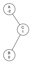
The diagram below shows us that after the left rotation we are now out of balance the other way. If we do a right rotation to correct the situation we are right back where we started.
After a left rotation, the tree is out of balance in the other direction
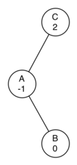
To correct this problem we must use the following set of rules:
- If a subtree needs a left rotation to bring it into balance, first check the balance factor of the right child. If the right child is left heavy then do a right rotation on right child, followed by the original left rotation.
- If a subtree needs a right rotation to bring it into balance, first check the balance factor of the left child. If the left child is right heavy then do a left rotation on the left child, followed by the original right rotation.
The diagram below shows how these rules solve the dilemma we encountered above. Starting with a right rotation around node C puts the tree in a position where the left rotation around A brings the entire subtree back into balance.
A right rotation followed by a left rotation
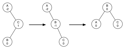
The code that implements these rules can be found in our rebalance method, which is shown below. Rule number 1 from above is implemented by the if statement starting on line 2. Rule number 2 is implemented by the elif statement starting on line 8.
def rebalance(self, node):
if node.balance_factor < 0 and node.right:
if node.right.balance_factor > 0:
self.rotate_right(node.right)
self.rotate_left(node)
else:
self.rotate_left(node)
elif node.balance_factor > 0 and node.left:
if node.left.balance_factor < 0:
self.rotate_left(node.left)
self.rotate_right(node)
else:
self.rotate_right(node)
By keeping the tree in balance at all times, we can ensure that the get method will run in order O(log2[n]) time. But the question is at what cost to our put method? Let us break this down into the operations performed by put. Since a new node is inserted as a leaf, updating the balance factors of all the parents will require a maximum of log2[n] operations, one for each level of the tree. If a subtree is found to be out of balance a maximum of two rotations are required to bring the tree back into balance. But, each of the rotations works in O(1) time, so even our put operation remains O(log2[n]).
At this point we have implemented a functional AVL-Tree, unless you need the ability to delete a node. We leave the deletion of the node and subsequent updating and rebalancing as an exercise for you.
Over the past few sections we have looked at several data structures that can be used to implement the map abstract data type. A binary Search on a list, a hash table, a binary search tree, and a balanced binary search tree. To conclude this section, let’s summarize the performance of each data structure for the key operations defined by the map ADT.
operation | Sorted List | Hash Table | Binary Search Tree | AVL Tree |
put | O(n) | O(1) | O(n) | O(log2n) |
get | O(log2n)) | O(1) | O(n) | O(log2n) |
in | O(log2n) | O(1) | O(n) | O(log2n) |
del | O(n) | O(1) | O(n) | O(log2n) |
9. முனை-ஓரம் தரவமைப்பு - Graphs
9.1 அறிமுகம் - Introduction to Graphs
இந்த அத்தியாயத்தில் நாம் முனை-ஓரம் அடைவுப் (graphs) படிப்போம். கடந்த அத்தியாயத்தில் நாம் படித்த மர தரவமைப்பை விட முனை-ஓரம் அடைவுகள் மிகவும் பொதுவான அமைப்பு ஆகும். உண்மையில் நீங்கள் ஒரு மர தரவமைப்பை ஒரு சிறப்பு வகையான முனை-ஓரம் அடைவாக நினைக்கலாம். சாலைகளின் அமைப்புகள், நகரத்திலிருந்து நகரத்திற்கு விமான பயணங்கள்,இணையம் எவ்வாறு இணைக்கப்பட்டுள்ளது என்பது அல்லது கணினி அறிவியலில் ஒரு முக்கியப் படிப்பை முடிக்க நீங்கள் எடுக்க வேண்டிய வகுப்புகளின் வரிசை உட்பட நமது உலகத்தைப் பற்றிய பல சுவாரஸ்யமான விஷயங்களைக் குறிக்க முனை-ஓரம் அடைவு பயன்படுத்தப்படலாம். ஒரு பிரச்சனைக்கு ஒரு நல்ல பிரதிநிதித்துவம் கிடைத்தவுடன், சில தரநிலையான முனை-ஓரம் அடைவு வழிமுறைகளைப் பயன்படுத்தி தீர்க்கலாம்.இல்லையேல் அது மிகவும் கடினமான பிரச்சனையாகத் தோன்றும்.
அத்தியாயம் முழுவதும் முனை-ஓரம் அடைவு பற்றி நாம் துல்லியமாக பேச அனுமதிக்கும் சில வரையறைகளை கீழே அறிமுகப்படுத்துகிறோம்.
உச்சி (Vertex)
ஒரு உச்சம் ஆனது முனை-ஓரம் அடைவின் அடிப்படை அலகாகும் இது “node” எனவும் அழைக்கப்படும்.இது ஒரு பெயரைக் கொண்டிருக்க முடியும் அதை நாங்கள் “key” என்று அழைப்போம். உச்சமானது “payload.” என அழைக்கப்படும் மேலதிக தகவல்களைக் கொண்டிருக்கலாம்.
விளிம்பு (Edge)
ஒரு விளிம்பு என்பது முனை-ஓரம் அடைவின் மற்றொரு அடிப்படை பகுதியாகும். ஒரு விளிம்பு இரண்டு உச்சிகளை இணைத்து அவற்றுக்கிடையே ஒரு தொடர்பு இருப்பதைக் காட்டும் விளிம்புகள் ஒரு வழி அல்லது இரு வழி ஆனதாக இருக்கலாம். ஒரு முனை-ஓரம் அடைவில் உள்ள விளிம்புகள் அனைத்தும் ஒரு வழியாக இருந்தால், நாங்கள் அதை directed graph அல்லது digraph என்று சொல்கிறோம்
எடை (Weight)
ஒரு உச்சியில் இருந்து மற்றொன்றுக்குச் செல்ல ஒரு செலவு இருக்கிறது என்பதைக் காட்ட விளிம்புகளின் எடை அளக்கப்படலாம் . உதாரணமாக ஒரு நகரத்தை இன்னொரு நகரத்துடன் இணைக்கும் சாலைகளின் முனை-ஓரம் அடைவில் , விளிம்பின் எடை இரண்டு நகரங்களுக்கிடையேயான தூரத்தைக் குறிக்கும்.
எங்களிடமுள்ள உள்ள வரையறைகளை வைத்து நாம் ஒரு முனை-ஓரம் அடைவினை முறையாக வரையறுக்கலாம். ஒரு முனை-ஓரம் அடைவு G =(V,E) ஆக இருக்கும் போது G என குறிப்பிட முடியும்.முனை-ஓரம் அடைவு G இல் V ஆனது உச்சிகளும் E ஆனது விளிம்புகளுமாகும்.ஒவ்வொரு விளிம்பும் ஒரு tuple (v,w) ஆகும் எப்போதென்றால் w,v என்பன V இல் உள்ள போதாகும்.எடையினைப் பிரதிநிதித்துவப்படுத்த நாம் மூன்றாவது கூறினை விளிம்பு tuple இற்கு சேர்க்கின்றோம்.ஒரு துணை முனை-ஓரம் அடைவு s ஆனது ஒரு தொகுதி e எனப்படும் விளிம்புகளையும், v எனப்படும் உச்சிகளையும் கொண்டிருக்கும்.e ஆனது E இன் ஒரு துணைப்பிரிவாகும்.அதேபோல் v ஆனது V இன் ஒரு துணைப்பிரிவாகும்.
கீழே உள்ள முனை-ஓரம் அடைவு எளிய எடையுள்ள ஒரு வழி முனை-ஓரம் அடைவின் மற்றொரு உதாரணத்தைக் காட்டுகிறது. முறையாக நாம் இந்த முனை-ஓரம் அடைவினை ஆறு உச்சிகளின் தொகுப்பாகக் குறிப்பிடலாம்:
V={V0,V1,V2,V3,V4,V5} and the set of nine edges:
E={(v0,v1,5),(v1,v2,4),(v2,v3,9),(v3,v4,7),(v4,v0,1),(v0,v5,2),(v5,v4,8),(v3,v5,3),(v5,v2,1)}
A simple example of a directed graph
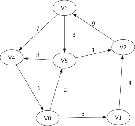
மேலே உள்ள உதாரணம் மற்ற இரண்டு முக்கிய முனை-ஓரம் அடைவுச் சொற்களை விளக்க உதவுகிறது:
வழி (Path)
ஒரு முனை-ஓரம் அடைவில் உள்ள வழி என்பது விளிம்புகளால் இணைக்கப்பட்ட உச்சிகளாகும். முறையாக நாங்கள் ஒரு பாதையை w1,w2,...,wn என வரையறுப்போம்; அதாவது 1≤ i ≤n−1 என்றபடியாக உள்ளவரை (wi,wi+1) ∈ E. எடை இல்லாத வழியின் நீளம் என்பது பாதையில் உள்ள விளிம்புகளின் எண்ணிக்கை ஆகும்.குறிப்பாக $$ n-1 $$. ஆகும்.எடை உள்ள வழியின் நீளம் என்பது அனைத்து விளிம்புகளின் எடைகளின் கூட்டுத்தொகையாகும். உதாரணமாக மேலே உள்ள முனை-ஓரம் அடைவில் V3 இலிருந்து V1 வரை வழியில் என்ற உச்சிகளும் (V3,V4,V0,V1), {(v3,v4,7),(v4,v0,1),(v0,v1,5)} என்ற விளிம்புகளும் உள்ளன.
முழு நிலை தொடர் வரிசை (Cycle)
ஒரு முழு நிலை தொடர் வரிசை என்பது முனை-ஓரம் அடைவில் ஒரு வழி ஒரு உச்சசியில் ஆரம்பித்து அதே உச்சியில் முடிவடைவதாகும்.எடுத்துக்காட்டாக, மேலே உள்ள முனை-ஓரம் அடைவில் வழி (V5, V2, V3, V5) என்பது ஒரு முழு நிலை தொடர் வரிசையாகும்.முழு நிலை தொடர் வரிசை இல்லாத முனை-ஓரம் அடைவு acyclic முனை-ஓரம் அடைவு என அழைக்கப்படும் .முழு நிலை தொடர் வரிசை இல்லாத ஒரு directed முனை-ஓரம் அடைவு directed acyclic முனை-ஓரம் அடைவு அல்லது DAG என அழைக்கப்படும். ஒரு சிக்கலானது DAG இனை பிரதிநிதித்துவப்படுத்தினால் பல சிக்கல்களைத் தீர்க்க முடிவதை நாங்கள் பார்க்கலாம்.
The Graph Abstract Data Type
முனை-ஓரம் அடைவுச் சுருக்க தரவு வகை (ADT) பின்வருமாறு வரையறுக்கப்படுகிறது:
- Graph() புதிய, வெறுமையான முனை-ஓரம் அடைவினை உருவாக்கவும்.
- add_vertex(vertex) முனை-ஓரம் அடைவின் உச்சிகளில் புதிய உச்சியை சேர்க்கும்
- add_edge(from_vertex, to_vertex) இரண்டு உச்சிகளை இணைக்கும் புதிய, இயக்கிய விளிம்பை சேர்க்கும்
- add_edge(from_vertex, to_vertex, weight) இரண்டு உச்சிகளை இணைக்கும் புதிய, எடையுள்ள, இயக்கிய விளிம்பை சேர்க்கும்
- get_vertex(key) key` எனப் பெயரிடப்பட்ட உச்சியை முனை-ஓரம் அடைவினில் தேடும் .
- get_vertices() முனை-ஓரம் அடைவினில் உள்ள எல்லா உச்சிகளின் பட்டியலைத் தரும்
- in முனை-ஓரம் அடைவினில் உச்சிக்கான அறிக்கை உண்டெனில் true ஐயும் இல்லையெனில் false ஐயும் தரும்.
ஒரு வரைபடத்திற்கான முறையான வரையறையுடன் தொடங்கி, பைத்தானில் ADT வரைபடத்தை நாம் செயல்படுத்த பல வழிகள் உள்ளன. மேலே விவரிக்கப்பட்ட ADT ஐச் செயல்படுத்த வெவ்வேறு பிரதிநிதித்துவங்களைப் பயன்படுத்துவதில் வர்த்தகம் இருப்பதைக் காண்போம். ஒரு வரைபடத்தின் இரண்டு நன்கு அறியப்பட்ட செயலாக்கங்கள் உள்ளன அவை adjacency matrix மற்றும் adjacency list ஆகும். இந்த இரண்டு விருப்பங்களையும் நாங்கள் விளக்குவோம், பின்னர் ஒன்றை பைதான் வகுப்பாக செயல்படுத்துவோம்.
9.2 முனை ஓரம் தரவமைப்பின் குறிமுறை - Representing a Graph
இந்த பிரிவில் முனை-ஓரம் அடைவின் இரண்டு பொதுவான சுருக்க பிரதிநிதித்துவங்களைப் பார்ப்போம்: அவை அடுத்துள்ள அச்சு வார்ப்புரு மற்றும் துரதிருஷ்டவசமாக அடுத்துள்ள" பட்டியல்". மாற்றக்கூடிய பட்டியல் உண்மையில் ஒரு ஒப்பீடு ஆகும், எனவே இந்த பிரிவில் அருகிலுள்ள பட்டியலின் பைத்தானில் இரண்டு சாத்தியமான பிரதிநிதித்துவங்களையும் நாங்கள் கருதுகிறோம்: ஒரு பொருள் சார்ந்த அணுகுமுறை பைதான் dict அதன் அடிப்படை தரவு வகையாகவும், ஒன்று நேரடியாக ஒரு தெளிவான கட்டளையைப் பயன்படுத்துகிறது.
முனை-ஓரம் அடைவுகளை பிரதிநிதித்துவப்படுத்த பல வழிகளை அறிந்திருப்பது பயனுள்ளது, ஏனெனில் நீங்கள் அவற்றை எல்லா இடங்களிலும் சந்திப்பீர்கள். இருந்தாலும், அடுத்துள்ள பட்டியல் பிரதிநிதித்துவத்தை தூய முனை-ஓரம் அடைவு வகையைப் பயன்படுத்தி (பைத்தானில் ஒரு dict போன்றவை) மிகவும் உள்ளுணர்வு மற்றும் நெகிழ்வானதாக நாங்கள் பார்க்கிறோம்.
அண்மைய அச்சு வார்ப்புரு (The Adjacency Matrix)
ஒரு முனை-ஓரம் அடைவினை செயல்படுத்த எளிதான வழிகளில் ஒன்று இரு பரிமாண அச்சு வார்ப்புருக்களைப் பயன்படுத்துவது. இந்த அச்சு வார்ப்புருக்களின் செயல்பாட்டில், வரிசைகள் மற்றும் நெடுவரிசைகள் ஒவ்வொன்றும் முனை-ஓரம் அடைவில் ஒரு உச்சநிலையைக் குறிக்கின்றன. வரிசை v மற்றும் நெடுவரிசை சந்திப்பில் உள்ள கலத்தில் சேமிக்கப்பட்ட மதிப்பு, உச்சி v லிருந்து உச்சி w வரை ஒரு விளிம்பு இருக்கிறதா என்பதைக் குறிக்கிறது. இரண்டு உச்சிகள் ஒரு விளிம்பால் இணைக்கப்படும்போது, அதை adjacent என அழைக்கின்றோம். கீழே உள்ள முனை-ஓரம் அடைவு நாம் முன்பு வழங்கிய எடுத்துக்காட்டு முனை-ஓரம் அடைவுற்கு அருகிலுள்ள அச்சு வார்ப்புருக்களை விளக்குகிறது. ஒரு கலத்தில் உள்ள மதிப்பு விளிம்பில் இருந்து விளிம்பின் எடையைக் குறிக்கிறது.
An adjacency matrix representation for a graph
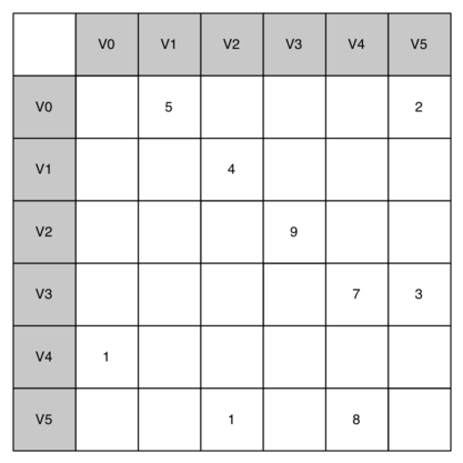
அருகிலுள்ள அச்சு வார்ப்புருக்களின் நன்மை என்னவென்றால், இது எளிதானது, மேலும் சிறிய முனை-ஓரம் அடைவுகளுக்கு எந்த முனைகள் மற்ற முனைகளுடன் இணைக்கப்பட்டுள்ளன என்பதைப் பார்ப்பது எளிது. இருப்பினும், அச்சு வார்ப்புருக்களில் உள்ள பெரும்பாலான செல்கள் காலியாக இருப்பதை கவனிக்கவும். பெரும்பாலான செல்கள் காலியாக இருப்பதால் இந்த அச்சு வார்ப்புருக்கள் "அரிதானது(sparse)" என்று சொல்கிறோம். ஒரு அச்சு வார்ப்புரு என்பது குறைவான தரவுகளைச் சேமிப்பதற்கான மிகச் சிறந்த வழி அல்ல. உண்மையில், பைத்தானில் மேலே உள்ளதைப் போன்ற ஒரு அச்சு வார்ப்புரு கட்டமைப்பை உருவாக்க நீங்கள் உங்கள் வழியை விட்டு வெளியேற வேண்டும்
விளிம்புகளின் எண்ணிக்கை பெரியதாக இருக்கும்போது அருகிலுள்ள அச்சு வார்ப்புரு ஒரு முனை-ஓரம் அடைவிற்கு ஒரு நல்ல செயல்படுத்தல் ஆகும். ஆனால் பெரியது என்று நாம் என்ன சொல்கிறோம்? அச்சு வார்ப்புருவை நிரப்ப எத்தனை விளிம்புகள் தேவைப்படும்? முனை-ஓரம் அடைவில் ஒவ்வொரு உச்சிக்கும் ஒரு வரிசை மற்றும் ஒரு நெடுவரிசை இருப்பதால், அச்சு வார்ப்புருவை நிரப்ப தேவையான விளிம்புகளின் எண்ணிக்கை |V|2. ஒவ்வொரு முனையையும் மற்ற ஒவ்வொரு உச்சியிலும் இணைக்கும்போது ஒரு அச்சு வார்ப்புரு நிரம்பியுள்ளது. இந்த வகையான இணைப்பை அணுகும் சில உண்மையான பிரச்சினைகள் உள்ளன. இந்த பிரிவில் நாம் பார்க்கும் சிக்கல்கள் அனைத்தும் குறைவாகவே இணைக்கப்பட்டுள்ள முனை-ஓரம் அடைவுகளை உள்ளடக்கியது..
அண்மைய பட்டியல் (The Adjacency List)
இணைக்கப்பட்ட முனை-ஓரம் அடைவை செயல்படுத்த மேலதிக இடத்திற்க்கான மிகத் திறமையான வழி துரதிருஷ்டவசமாக பெயரிடப்பட்ட அருகிலுள்ள பட்டியல் கட்டமைப்பைப் பயன்படுத்துவது ஆகும்.அருகிலுள்ள பட்டியல் செயல்பாட்டில், முனை-ஓரம் அடைவுப் பொருளில் உள்ள அனைத்து நுனிகளின் முதன்மைத் தொகுப்பை நாங்கள் வைத்திருக்கிறோம், பின்னர் முனை-ஓரம் அடைவில் உள்ள ஒவ்வொரு உச்சநிலைப் பொருளும் அது இணைக்கப்பட்ட மற்ற உச்சங்களின் பட்டியலைப் பராமரிக்கிறது. உச்சிகள் வகுப்பைச் செயல்படுத்துவதில், எங்கள் முதன்மைத் தொகுப்பாக பட்டியலை விட ஒரு தொடர்புறு அணியைப் பயன்படுத்துவோம், அங்கு தொடர்புறு அணியின் விசைகள், உச்சிகள் , மற்றும் மதிப்புகளின் எடைகள் ஆகும் . கீழே உள்ள முனை-ஓரம் அடைவு நாம் விவாதித்த உதாரண முனை-ஓரம் அடைவின் அருகிலுள்ள பட்டியல் பிரதிநிதித்துவத்தைக் காட்டுகிறது.
An adjacency list representation of a graph
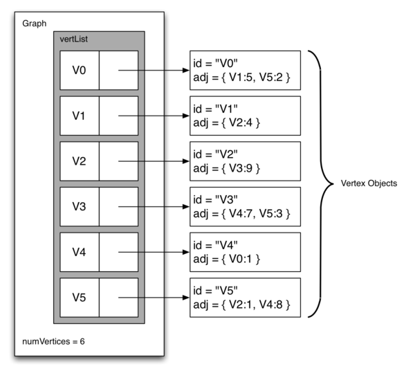
அருகிலுள்ள பட்டியல் செயல்பாட்டின் நன்மை என்னவென்றால், இது ஒரு சிறிய முனை-ஓரம் அடைவை சுருக்கமாக பிரதிநிதித்துவப்படுத்த அனுமதிக்கிறது. அருகிலுள்ள பட்டியல் ஒரு குறிப்பிட்ட உச்சத்துடன் நேரடியாக இணைக்கப்பட்டுள்ள அனைத்து இணைப்புகளையும் எளிதாகக் கண்டறிய அனுமதிக்கிறது.
பொருள் நோக்கு நிரலாக்கம் - An Object-Oriented Approach
தொடர்புறு அணியைப் பயன்படுத்தி, பைத்தானில் அருகிலுள்ள பட்டியலைச் செயல்படுத்துவது எளிது. இந்த செயல்பாட்டில் நாங்கள் இரண்டு வகுப்புகளை உருவாக்குகிறோம்: Graph உச்சிகளின் முதல்நிலைப் பட்டியலை வைத்திருக்கும்.Vertexமுனை-ஓரம் அடைவில் உள்ள ஒவ்வொரு உச்சியையும் குறிக்கும்.
ஒவ்வொரு Vertex உம் ஒரு தொடர்புறு அணியைப் பயன்படுத்தி அது இணைக்கப்பட்டுள்ள உச்சிகள் மற்றும் ஒவ்வொரு விளிம்பின் எடையையும் கண்காணிக்கின்றன. விளிம்பு எடையுடன் நாங்கள் அக்கறை கொள்ளவில்லை என்றால், தொடர்புறு அணியின் இடத்தில் ஒரு தொகுப்பைப் பயன்படுத்தலாம். இந்த தொடர்புறு அணி neighbors என்று அழைக்கப்படுகிறது.
கீழே உள்ள குறியீட்டில், add_neighbor முறை இந்த உச்சியில் இருந்து இன்னொரு இணைப்பைச் சேர்க்கப் பயன்படுகிறது. get_connections முறை அருகிலுள்ள பட்டியலில் உள்ள அனைத்து முனைகளையும் வழங்குகிறது,neighbors இனால் மாறிகள் பிரதிநிதித்துவப்படுத்தப்படும்.get_weight முறை இந்த உச்சியிலிருந்து ஒரு செயலுருவாகக் கடந்து செல்லும் விளிம்பின் எடையை தருகிறது.
class Vertex(object):
def __init__(self, key):
self.key = key
self.neighbors = {}
def add_neighbor(self, neighbor, weight=0):
self.neighbors[neighbor] = weight
def __str__(self):
return '{} neighbors: {}'.format(
self.key,
[x.key for x in self.neighbors]
)
def get_connections(self):
return self.neighbors.keys()
def get_weight(self, neighbor):
return self.neighbors[neighbor]
கீழே காட்டப்பட்டுள்ள Graph வகுப்பில்,உச்சிகளின் பெயர்களை உச்சிகளின் பொருட்களுக்கு ஒப்பீடு செய்யும் ஒரு தொடருறு அணி உள்ளது.Graph முறையானது முனை-ஓரம் அடைவில் ஒரு உச்சியை சேர்க்கவும் மற்றும் ஒரு உச்சியை இன்னொரு உச்சியுடன் இணைக்கவும் பயன்படுகின்றது.get_vertices முறையானது முனை-ஓரம் அடைவில் உள்ள எல்லா உச்சிகளின் பெயரையும் தருகின்றது.கூடுதலாக, ஒரு குறிப்பிட்ட முனை-ஓரம் அடைவில் உள்ள அனைத்து உச்சசிப் பொருட்களின் மீதும் சுலபமாகச் செய்யல்படக்கூடிய __iter__முறையை நாங்கள் செயல்படுத்தியுள்ளோம். இரண்டு முறைகளும் ஒரு முனை-ஓரம் அடைவில் உள்ள உச்சவரம்புகளை பெயரால் அல்லது பொருள்களால் மீண்டும் செய்ய உங்களை அனுமதிக்கிறது.
class Graph(object):
def __init__(self):
self.verticies = {}
def add_vertex(self, vertex):
self.verticies[vertex.key] = vertex
def get_vertex(self, key):
try:
return self.verticies[key]
except KeyError:
return None
def __contains__(self, key):
return key in self.verticies
def add_edge(self, from_key, to_key, weight=0):
if from_key not in self.verticies:
self.add_vertex(Vertex(from_key))
if to_key not in self.verticies:
self.add_vertex(Vertex(to_key))
self.verticies[from_key].add_neighbor(self.verticies[to_key], weight)
def get_vertices(self):
return self.verticies.keys()
def __iter__(self):
return iter(self.verticies.values())
இப்போது வரையறுக்கப்பட்ட Graphமற்றும் Vertex வகுப்புகளைப் பயன்படுத்தி,பின்வரும் பைதான் அமர்வு எங்கள் எடுத்துக்காட்டு வரைபடத்தை உருவாக்குகிறது.முதலில் 0 முதல் 5 வரையிலான ஆறு உச்சிகளை உருவாக்குகிறோம், பின்னர் நாம் உச்சிகளின் தொடர்புறு அணியைக் காண்பிப்போம். 0 முதல் 5 வரையான ஒவ்வொரு சாவிக்கும் Vertex இன் மாதிரியை உருவாக்கியுள்ளோம் என்பதை கவனிக்கவும். அடுத்து, உச்சிகளை ஒன்றாக இணைக்கும் விளிம்புகளைச் சேர்க்கிறோம். இறுதியாக, கூடு மீள்செய்தலானது முனை-ஓரம்-அடைவில் உள்ள ஒவ்வொரு விளிம்பும் சரியாக சேமிக்கப்பட்டுள்ளதா என்பதை சரிபார்க்கிறது.
>>> g = Graph()
>>> for i in range(6):
... g.add_vertex(Vertex(i))
>>> g.verticies
{0: <adjGraph.Vertex instance at 0x41e18>,
1: <adjGraph.Vertex instance at 0x7f2b0>,
2: <adjGraph.Vertex instance at 0x7f288>,
3: <adjGraph.Vertex instance at 0x7f350>,
4: <adjGraph.Vertex instance at 0x7f328>,
5: <adjGraph.Vertex instance at 0x7f300>}
>>> g.add_edge(0, 1, 5)
>>> g.add_edge(0, 5, 2)
>>> g.add_edge(1, 2, 4)
>>> g.add_edge(2, 3, 9)
>>> g.add_edge(3, 4, 7)
>>> g.add_edge(3, 5, 3)
>>> g.add_edge(4, 0, 1)
>>> g.add_edge(5, 4, 8)
>>> g.add_edge(5, 2, 1)
>>> for v in g:
... for w in v.get_connections():
... print('{} -> {}'.format(v.key, w.key))
...
0 -> 5
0 -> 1
1 -> 2
2 -> 3
3 -> 4
3 -> 5
4 -> 0
5 -> 4
5 -> 2
நேரடியாக தொடர்புறு அணியைப் பயன்படுத்துதல் (Using Dictionaries Directly)
மரங்களின் முனை மற்றும் விளிம்புகளின் பிரதிநிதித்துவத்தைப் போலவே, எங்கள் முனை-ஓரம் அடைவின் அடிப்படைக் கட்டமைப்பை நாம் மேலே உள்ளதைப் போல வகுப்புகளுடன் போர்த்துவது பயனுள்ளது என்று நீங்கள் யோசிக்கலாம். இது சூழலைப் பொறுத்தது, ஆனால் எங்கள் பொதுவான விருப்பம் உண்மையில் தரவு கட்டமைப்போடு நேரடியாக வேலை செய்வதாகும். அவ்வாறு செய்வதன் மூலம் ஒரு முனை-ஓரம் அடைவை மிக எளிதாக அச்சிடலாம் அல்லது மற்றபடி பிழைதிருத்தம் செய்யலாம், ஒரு முனை-ஓரம் அடைவை நேரடி கலப்பு வகையாக உருவாக்கலாம், மேலும் ஒரு முனை-ஓரம் அடைவை JSON க்கு வரிசைப்படுத்தலாம்.
மேலே உள்ள எடுத்துக்காட்டு முனை-ஓரம் அடைவு இப்படி இருக்கும்:
{
0: {1: 5, 5: 2},
1: {2: 4},
2: {3: 9},
3: {4: 7, 5: 3},
4: {0: 1},
5: {4: 8}
}
அத்தியாயத்தின் எஞ்சிய பகுதிகளுக்கு, பெரும்பாலான சந்தர்ப்பங்களில் நேரடியாக தொடர்புறு அணியைப் பயன்படுத்துவோம்.
9.3 சொல் ஏணிகள் விளையாட்டு - Word Ladders
To begin our study of graph algorithms let’s consider the following puzzle called a word ladder. Transform the word “FOOL” into the word “SAGE”. In a word ladder puzzle you must make the change occur gradually by changing one letter at a time. At each step you must transform one word into another word, you are not allowed to transform a word into a non-word. The word ladder puzzle was invented in 1878 by Lewis Carroll, the author of Alice in Wonderland. The following sequence of words shows one possible solution to the problem posed above.
FOOL
POOL
POLL
POLE
PALE
SALE
SAGE
There are many variations of the word ladder puzzle. For example you might be given a particular number of steps in which to accomplish the transformation, or you might need to use a particular word. In this section we are interested in figuring out the smallest number of transformations needed to turn the starting word into the ending word.
Not surprisingly, since this chapter is on graphs, we can solve this problem using a graph algorithm. Here is an outline of where we are going:
- Represent the relationships between the words as a graph.
- Use the graph algorithm known as breadth first search to find an efficient path from the starting word to the ending word.
Building the Word Ladder Graph
Our first problem is to figure out how to turn a large collection of words into a graph. What we would like is to have an edge from one word to another if the two words are only different by a single letter. If we can create such a graph, then any path from one word to another is a solution to the word ladder puzzle. The illustration below shows a small graph of some words that solve the FOOL to SAGE word ladder problem. Notice that the graph is an undirected graph and that the edges are unweighted.
A small word ladder graph
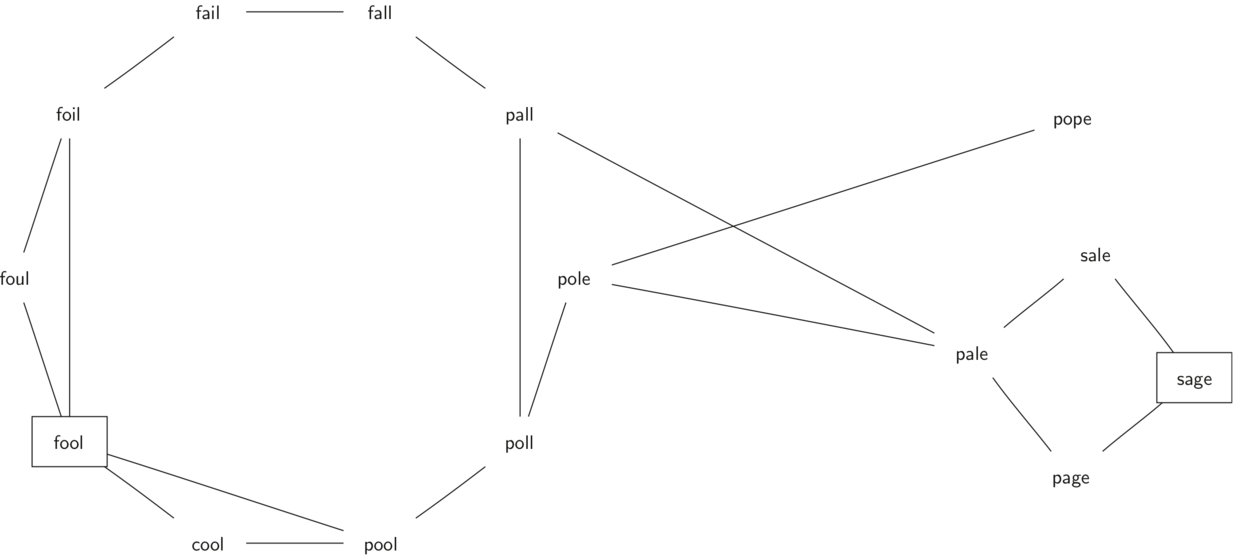
We could use several different approaches to create the graph we need to solve this problem. Let’s start with the assumption that we have a list of words that are all the same length. As a starting point, we can create a vertex in the graph for every word in the list. To figure out how to connect the words, we could compare each word in the list with every other. When we compare we are looking to see how many letters are different. If the two words in question are different by only one letter, we can create an edge between them in the graph. For a small set of words that approach would work fine; however let’s suppose we have a list of 5,110 words. Roughly speaking, comparing one word to every other word on the list is an O(n2) algorithm. For 5,110 words, n2 is more than 26 million comparisons.
We can do much better by using the following approach. Suppose that we have a huge number of buckets, each of them with a four-letter word on the outside, except that one of the letters in the label has been replaced by an underscore. For example we might have a bucket labeled “pop_.” As we process each word in our list we compare the word with each bucket, using the ‘_’ as a wildcard, so both “pope” and “pops” would match “pop_.” Every time we find a matching bucket, we put our word in that bucket. Once we have all the words in the appropriate buckets we know that all the words in the bucket must be connected.
Word buckets for words that are different by one letter
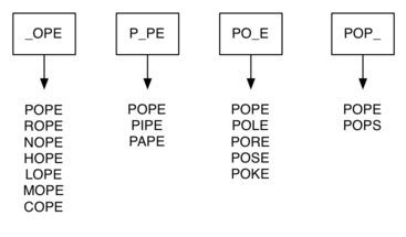
In Python, we can implement the scheme we have just described by using a dictionary. The labels on the buckets we have just described are the keys in our dictionary. The value stored for that key is a list of words. Once we have the dictionary built we can create the graph. We start our graph by creating a vertex for each word in the graph. Then we create edges between all the vertices we find for words found under the same key in the dictionary.
Below is an example of Python code implementing this strategy. In this case, we use a dictionary mapping vertices (words) to sets of the vertices that can be reached by changing one letter in that word.
from collections import defaultdict
from itertools import product
import os
def build_graph(words):
buckets = defaultdict(list)
graph = defaultdict(set)
for word in words:
for i in range(len(word)):
bucket = '{}_{}'.format(word[:i], word[i + 1:])
buckets[bucket].append(word)
# add vertices and edges for words in the same bucket
for bucket, mutual_neighbors in buckets.items():
for word1, word2 in product(mutual_neighbors, repeat=2):
if word1 != word2:
graph[word1].add(word2)
graph[word2].add(word1)
return graph
def get_words(vocabulary_file):
for line in open(vocabulary_file, 'r'):
yield line[:-1] # remove newline character
vocabulary_file = os.path.join(os.path.dirname(__file__), 'vocabulary.txt')
word_graph = build_graph(get_words(vocabulary_file))
# word_graph['FOOL']
# set(['POOL', 'WOOL', 'FOWL', 'FOAL', 'FOUL', ... ])
Since this is our first real-world graph problem, you might be wondering how sparse is the graph? The list of four-letter words we have for this problem is 5,110 words long. If we were to use an adjacency matrix, the matrix would have 5,110 * 5,110 = 26,112,100 cells. The graph constructed by the build_graph function has exactly 53,286 edges, so the matrix would have only 0.20% of the cells filled! That is a very sparse matrix indeed.
Implementing breadth first search
With the graph constructed we can now turn our attention to the algorithm we will use to find the shortest solution to the word ladder problem. The graph algorithm we are going to use is called the “breadth first search” algorithm. Breadth first search (BFS) is one of the easiest algorithms for searching a graph. It also serves as a prototype for several other important graph algorithms that we will study later.
Given a graph GGG and a starting vertex sss, a breadth first search proceeds by exploring edges in the graph to find all the vertices in GGG for which there is a path from sss. The remarkable thing about a breadth first search is that it finds all the vertices that are a distance k from sss before it finds any vertices that are a distance k+1. One good way to visualize what the breadth first search algorithm does is to imagine that it is building a tree, one level of the tree at a time. A breadth first search adds all children of the starting vertex before it begins to discover any of the grandchildren.
The breadth first search algorithm shown below uses the adjacency list graph representation we developed earlier. In addition it uses a queue at a crucial point as we will see, to decide which vertex to explore next, and also to maintain a record of the depth to which we have traversed at any point.
BFS starts by initializing a set to retain a record of which vertices have been visited already. Next, we initialize a queue (in this case utilizing the deque type from Python’s collections module) which will contain all paths from our starting vertex that we have explored as our algorithm progress. As such we initialize it with a list containing just our starting vertex.
The next step is to begin to systematically grow the paths one at a time, starting from the path at the front of the queue, in each case taking one more step from the vertex last explored.
Once we have popped from our queue a path to continue exploring and retrieved the last the vertex visited from that path, we retrieve its neighbors from our graph, remove those vertices that we know have already been visited, then for each of the remaining (unvisited) neighbors do two things:
- Add the vertex to visited
- Add a path consisisting of the path so far plus the vertex
Adding the new vertex effectively schedules it for further exploration, but not until all the other vertices on the adjacency list have been explored.
from collections import deque
def traverse(graph, starting_vertex):
visited = set()
queue = deque([[starting_vertex]])
while queue:
path = queue.popleft()
vertex = path[-1]
yield vertex, path
for neighbor in graph[vertex] - visited:
visited.add(neighbor)
queue.append(path + [neighbor])
if __name__ == '__main__':
for vertex, path in traverse(word_graph, 'FOOL'):
if vertex == 'SAGE':
print ' -> '.join(path)
# FOOL -> FOOD -> FOLD -> SOLD -> SOLE -> SALE -> SAGE
Let’s look at how the traverse function would construct the breadth first tree corresponding to the word ladder graph we considered previously. Starting from fool we take all nodes that are adjacent to fool and add them to the tree. The adjacent nodes include pool, foil, foul, and cool. Each of these nodes are added to the queue of new nodes to expand. The illustration below shows the state of the in-progress tree along with the queue after this step.
The first step in the breadth first search
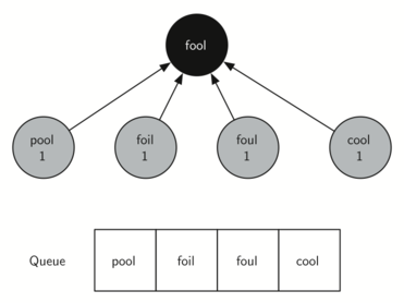
In the next step traverse removes the next node (pool) from the front of the queue and repeats the process for all of its adjacent nodes. However, when traverse examines the node cool, it finds that it has already been visited. This implies that there is a shorter path to cool. The only new node added to the queue while examining pool is poll. The new state of the tree and queue is shown below.
The second step in the breadth first search
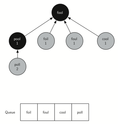
The next vertex on the queue is foil. The only new node that foil can add to the tree is fail. As traverse continues to process the queue, neither of the next two nodes add anything new to the queue or the tree. The illustration below shows the tree and the queue after expanding all the vertices on the second level of the tree.
Breadth first search tree after completing one level
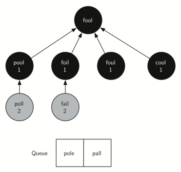
You should continue to work through the algorithm on your own so that you are comfortable with how it works. The illustration below shows the final breadth first search tree after all the vertices have been expanded.
Final breadth first search tree
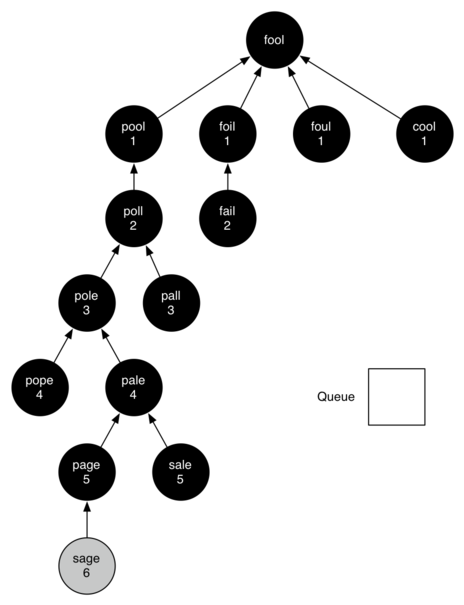
Breadth First Search Analysis
Before we continue with other graph algorithms let us analyze the run time performance of the breadth first search algorithm. The first thing to observe is that the while loop is executed, at most, one time for each vertex in the graph ∣V∣. You can see that this is true because a vertex must be white before it can be examined and added to the queue. This gives us O(V)for the while loop. The for loop, which is nested inside the while is executed at most once for each edge in the graph, ∣E∣. The reason is that every vertex is dequeued at most once and we examine an edge from node uuu to node vvv only when node uuu is dequeued. This gives us O(E) for the for loop. combining the two loops gives us O(V+E).
Of course doing the breadth first search is only part of the task. Following the links from the starting node to the goal node is the other part of the task. The worst case for this would be if the graph was a single long chain. In this case traversing through all of the vertices would be O(V). The normal case is going to be some fraction of ∣V∣|V|∣V∣ but we would still write O(V).
Finally, at least for this problem, there is the time required to build the initial graph. We leave the analysis of the build_graph function as an exercise for you.
9.4 A Knight’s Tour
The “knight’s tour” is a classic problem in graph theory, first posed over 1,000 years ago and pondered by legendary mathematicians including Leonhard Euler before finally being solved in 1823. We will use the knight’s tour problem to illustrate a second common graph algorithm called depth first search.
The knight’s tour puzzle is played on a chess board with a single chess piece, the knight. The object of the puzzle is to find a sequence of moves that allow the knight to visit every square on the board exactly once, like so:
One possible knight’s tour
One such sequence is called a “tour.” The upper bound on the number of possible legal tours for an eight-by-eight chessboard is known to be 1.305×10351.305 x 10^{35}1.305×1035; however, there are even more possible dead ends. Clearly this is a problem that requires some real brains, some real computing power, or both.
Once again we will solve the problem using two main steps:
- Represent the legal moves of a knight on a chessboard as a graph.
- Use a graph algorithm to find a path where every vertex on the graph is visited exactly once.
Building the Knight’s Tour Graph
To represent the knight’s tour problem as a graph we will use the following two ideas: Each square on the chessboard can be represented as a node in the graph. Each legal move by the knight can be represented as an edge in the graph.
We will use a Python dictionary to hold our graph, with the keys being tuples of coordinates representing the squares of the board, and the values being sets representing the valid squares to which a knight can move from that square.
To build the full graph for an n-by-n board we can use the Python function shown below. The build_graph function makes one pass over the entire board. At each square on the board the build_graph function calls a helper generator, legal_moves_from, to generate a list of legal moves for that position on the board. All legal moves are then made into undirected edges of the graph by adding the vertices appropriately to one anothers sets of legal moves.
from collections import defaultdict
def add_edge(graph, vertex_a, vertex_b):
graph[vertex_a].add(vertex_b)
graph[vertex_b].add(vertex_a)
def build_graph(board_size):
graph = defaultdict(set)
for row in range(board_size):
for col in range(board_size):
for to_row, to_col in legal_moves_from(row, col, board_size):
add_edge(graph, (row, col), (to_row, to_col))
return graph
The legal_moves_from generator below takes the position of the knight on the board and yields any of the eight possible moves that are still on the board.
MOVE_OFFSETS = (
(-1, -2), ( 1, -2),
(-2, -1), ( 2, -1),
(-2, 1),( 2, 1),
(-1, 2), ( 1, 2),
)
def legal_moves_from(row, col, board_size):
for row_offset, col_offset in MOVE_OFFSETS:
move_row, move_col = row + row_offset, col + col_offset
if 0 <= move_row < board_size and 0 <= move_col < board_size:
yield move_row, move_col
The illustration below shows the complete graph of possible moves on an eight-by-eight board. There are exactly 336 edges in the graph. Notice that the vertices corresponding to the edges of the board have fewer connections (legal moves) than the vertices in the middle of the board. Once again we can see how sparse the graph is. If the graph was fully connected there would be 4,096 edges. Since there are only 336 edges, the adjacency matrix would be only 8.2 percent full.
All legal moves for a knight on an 8x8 chessboard
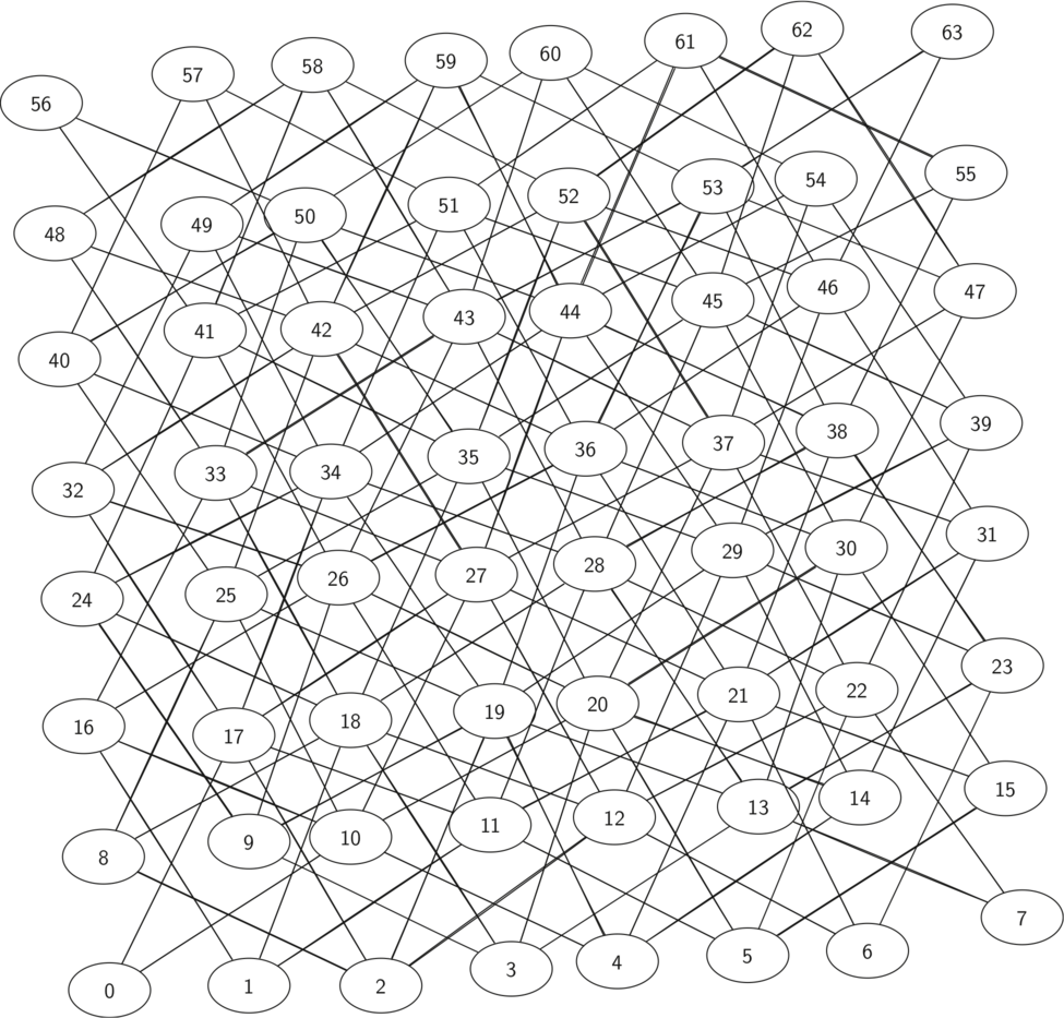
Implementing Knight’s Tour
The search algorithm we will use to solve the knight’s tour problem is called depth first search (DFS). Whereas the breadth first search algorithm discussed in the previous section builds a search tree one level at a time, a depth first search creates a search tree by exploring one branch of the tree as deeply as possible.
The depth first exploration of the graph is exactly what we need in order to find a path that has exactly 63 edges. We will see that when the depth first search algorithm finds a dead end (a place in the graph where there are no more moves possible) it backs up the tree to the next deepest vertex that allows it to make a legal move.
The find_solution_for function takes just two arguments: a board_size argument and a heuristic function, which you should ignore for now but to which we will return.
It then constructs a graph using the build_graph function described above, and for each vertex in the graph attempts to traverse depth first by way of the traverse function.
The traverse function is a little more interesting. It accepts a path, as a list of coordinates, as well as the vertex currently being considered. If the traversal has proceeded deep enough that we know that every square has been visited once, then we return the full path traversed.
Otherwise, we use our graph to look up the legal moves from the current vertex, and exclude the vertices that we know have already been visited, to determine the vertices that are yet_to_visit. At this point we recursively call traverse with each of the vertices to visit, along with the path to reach that vertex including the current vertex. If any of the recursive calls return a path, then that path is the return value of the outer call, otherwise we return None.
def first_true(sequence):
for item in sequence:
if item:
return item
return None
def find_solution_for(board_size, heuristic=lambda graph: None):
graph = build_graph(board_size)
total_squares = board_size * board_size
def traverse(path, current_vertex):
if len(path) + 1 == total_squares:
# including the current square, we've visited every square,
# so return the path as a solution
return path + [current_vertex]
yet_to_visit = graph[current_vertex] - set(path)
if not yet_to_visit:
# no unvisited neighbors, so dead end
return False
# try all valid paths from here
next_vertices = sorted(yet_to_visit, heuristic(graph))
return first_true(traverse(path + [current_vertex], vertex)
for vertex in next_vertices)
# try to find a solution from any square on the board
return first_true(traverse([], starting_vertex)
for starting_vertex in graph)
# find_solution_for(5) # => [(1, 3), (0, 1), (2, 0), (4, 1), (2, 2), ... ]
Let’s look at a simple example of an equivalent of this traverse function in action.
Start with vertex A
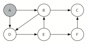
Explore B

Vertex C is a dead end
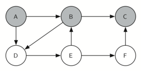
Backtrack to B
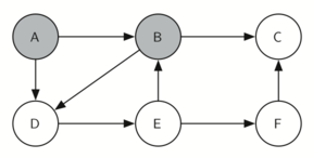
Explore D
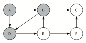
Explore E
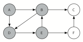
Explore F
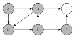
Finish
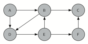
It is remarkable that our choice of data structure and algorithm has allowed us to straightforwardly solve a problem that remained impervious to thoughtful mathematical investigation for centuries.
With some modification, the algorithm can also be used to discover one of a number of “closed” (circular) tours, which can therefore be started at any square of the board:
A closed tour
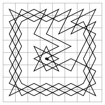
Knight’s Tour Analysis
There is one last interesting topic regarding the knight’s tour problem, then we will move on to the general version of the depth first search. The topic is performance. In particular, our algorithm is very sensitive to the method you use to select the next vertex to visit. For example, on a five-by-five board you can produce a path in about 1.5 seconds on a reasonably fast computer. But what happens if you try an eight-by-eight board? In this case, depending on the speed of your computer, you may have to wait up to a half hour to get the results! The reason for this is that the knight’s tour problem as we have implemented it so far is an exponential algorithm of size O(kN), where N is the number of squares on the chess board, and k is a small constant. The diagram below can help us visualize why this is so.
A search tree for the knight’s tour
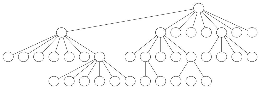
The root of the tree represents the starting point of the search. From there the algorithm generates and checks each of the possible moves the knight can make. As we have noted before the number of moves possible depends on the position of the knight on the board. In the corners there are only two legal moves, on the squares adjacent to the corners there are three and in the middle of the board there are eight. The diagram below shows the number of moves possible for each position on a board. At the next level of the tree there are once again between 2 and 8 possible next moves from the position we are currently exploring. The number of possible positions to examine corresponds to the number of nodes in the search tree.
Number of possible moves for each square
We have already seen that the number of nodes in a binary tree of height N is 2N+1−1. For a tree with nodes that may have up to eight children instead of two the number of nodes is much larger. Because the branching factor of each node is variable, we could estimate the number of nodes using an average branching factor. The important thing to note is that this algorithm is exponential: kN+1−1, where k is the average branching factor for the board. Let’s look at how rapidly this grows! For a board that is 5x5 the tree will be 25 levels deep, or N = 24 counting the first level as level 0. The average branching factor is k=3.8 So the number of nodes in the search tree is 3.825−1 or 3.12×10¹⁴ . For a 6x6 board, k=4.4, there are 1.5×10²³ nodes, and for a regular 8x8 chess board, k=5.25, there are 1.3×1046. Of course, since there are multiple solutions to the problem we won’t have to explore every single node, but the fractional part of the nodes we do have to explore is just a constant multiplier which does not change the exponential nature of the problem. We will leave it as an exercise for you to see if you can express k as a function of the board size.
Luckily there is a way to speed up the eight-by-eight case so that it runs in under one second. In the code sample below we show the code that speeds up the traverse. This function, called warnsdorffs_heuristic when passed as the heuristic function to find_solution_for above will cause the next_vertices to be sorted prioritizing those who which have the fewest subsequent legal moves.
This may seem counterintutitive; why not select the node that has the most available moves? The problem with using the vertex with the most available moves as your next vertex on the path is that it tends to have the knight visit the middle squares early on in the tour. When this happens it is easy for the knight to get stranded on one side of the board where it cannot reach unvisited squares on the other side of the board. On the other hand, visiting the squares with the fewest available moves first pushes the knight to visit the squares around the edges of the board first. This ensures that the knight will visit the hard-to- reach corners early and can use the middle squares to hop across the board only when necessary. Utilizing this kind of knowledge to speed up an algorithm is called a heuristic. Humans use heuristics every day to help make decisions, heuristic searches are often used in the field of artificial intelligence. This particular heuristic is called Warnsdorff’s heuristic, named after H. C. Warnsdorff who published his idea in 1823, becoming the first person to describe a procedure to complete the knight’s tour.
def warnsdorffs_heuristic(graph): #Given a graph, return a comparator function that prioritizes nodes #with the fewest subsequent moves def comparator(a, b): return len(graph[a]) - len(graph[b]) return comparator # find_solution_for(8, warnsdorffs_heuristic) # => [(7, 3), (6, 1), (4, 0), (2, 1), (0, 0), (1, 2), ... ] |
For fun, here is a very large (130×130130 x 130130×130) open knight’s tour created using Warnsdorff’s heuristic:
130x130 open tour
9.5 General Depth First Search
The knight’s tour is a special case of a depth first search where the goal is to create the deepest depth first tree, without any branches. The more general depth first search is actually easier. Its goal is to search as deeply as possible, connecting as many nodes in the graph as possible and branching where necessary.
It is even possible that a depth first search will create more than one tree. When the depth first search algorithm creates a group of trees we call this a depth first forest. As with the breadth first search our depth first search makes use of predecessor links to construct the tree. In addition, the depth first search will make use of two additional instance variables in the Vertex class. The new instance variables are the discovery and finish times. The discovery time tracks the number of steps in the algorithm before a vertex is first encountered. The finish time is the number of steps in the algorithm before a vertex is colored black. As we will see after looking at the algorithm, the discovery and finish times of the nodes provide some interesting properties we can use in later algorithms.
The code for our depth first search is shown below. We use a set to maintain a record of the nodes that have been visited as we recursively traverse through our sample graph. For each vertex, any neighboring vertices that have not yet been visited are traversed. This is much like our depth first traversal for our knight’s tour solution, except that we do not need to keep track of the path taken to reach every vertex, allowing us to more simply use our visited set.
We also introduce a traversal_times dictionary here in which the keys are vertices and the values we populate as dictionaries of the form {'discovery': m, 'finish': n}, where the m and n values are integers obtained by incrementing a counter before and after each time a new vertex is traversed.
from collections import defaultdict simple_graph = { 'A': ['B', 'D'], 'B': ['C', 'D'], 'C': [], 'D': ['E'], 'E': ['B', 'F'], 'F': ['C'] } def depth_first_search(graph, starting_vertex): visited = set() counter = [0] traversal_times = defaultdict(dict) def traverse(vertex): visited.add(vertex) counter[0] += 1 traversal_times[vertex]['discovery'] = counter[0] for next_vertex in graph[vertex]: if next_vertex not in visited: traverse(next_vertex) counter[0] += 1 traversal_times[vertex]['finish'] = counter[0] # in this case start with just one vertex, but we could equally # dfs from all_vertices to produce a dfs forest traverse(starting_vertex) return traversal_times traversal_times = depth_first_search(simple_graph, 'A') # => # { # 'A': { # 'discovery': 1, # 'finish': 12 # }, # 'B': { # 'discovery': 2, # 'finish': 11 # }, # 'C': { # 'discovery': 3, # 'finish': 4 # }, # 'D': { # 'discovery': 5, # 'finish': 10 # }, # 'E': { # 'discovery': 6, # 'finish': 9 # }, # 'F': { # 'discovery': 7, # 'finish': 8 # } # } |
The traverse method starts with a single vertex called and explores all of the neighboring unvisited vertices as deeply as possible. If you look carefully at the code for traverse and compare it to breadth first search, what you should notice is that the traverse algorithm is almost identical to breadth_first_search except that on the last line of the inner for loop, traverse calls itself recursively to continue the search at a deeper level, whereas breadth_first_search adds the node to a queue for later exploration. It is interesting to note that where breadth_first_search uses a queue, traverse uses a stack. You don’t see a stack in the code, but it is implicit in the recursive call to traverse.
The following sequence of figures illustrates the depth first search algorithm in action for a small graph. In these figures, the dotted lines indicate edges that are checked, but the node at the other end of the edge has already been added to the depth first tree. In the code this test is done by checking that the other node has been visited.
The search begins at vertex A of the graph (below). Since all of the vertices are unvisited at the beginning of the search the algorithm visits vertex A. The first step in visiting a vertex is to add it to the visited set, indicated here with a gray color, and the discovery time is set to 1. Since vertex A has two adjacent vertices (B, D) each of those need to be visited as well. We’ll make the arbitrary decision that we will visit the adjacent vertices in alphabetical order.
Constructing the depth first search tree

Vertex B is visited next (see below), so its color is set to gray and its discovery time is set to 2. Vertex B is also adjacent to two other nodes (C, D) so we will follow the alphabetical order and visit node C next.
Constructing the depth first search tree
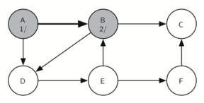
Visiting vertex C (see below) brings us to the end of one branch of the tree. After adding the node to visited and setting its discovery time to 3, the algorithm also determines that there are no adjacent vertices to C.
Constructing the depth first search tree
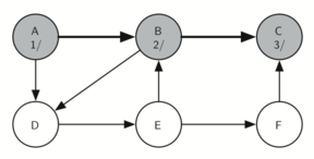
This means that we are done exploring node C and so we can color the vertex black, and set the finish time to 4. You can see the state of our search at this point below.
Constructing the depth first search tree
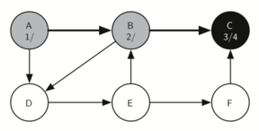
Since vertex C was the end of one branch we now return to vertex B and continue exploring the nodes adjacent to B. The only additional vertex to explore from B is D, so we can now visit D (below) and continue our search from vertex D.
Constructing the depth first search tree
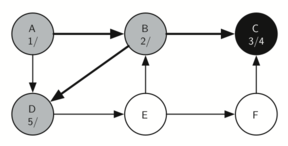
Vertex D quickly leads us to vertex E:
Constructing the depth first search tree
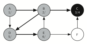
Vertex E has two adjacent vertices, B and F. Normally we would explore these adjacent vertices alphabetically, but since B has already been visited the algorithm recognizes that it should not visit B since doing so would put the algorithm in a loop! So exploration continues with the next vertex in the list, namely F.
Constructing the depth first search tree
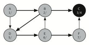
Vertex F has only one adjacent vertex, C, but since C has been visited there is nothing else to explore, and the algorithm has reached the end of another branch. From here on, you will see that the algorithm works its way back to the first node, setting finish times.
Constructing the depth first search tree
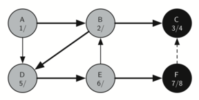
Constructing the depth first search tree
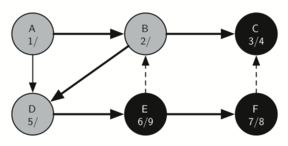
Constructing the depth first search tree
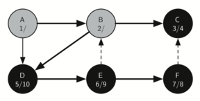
Constructing the depth first search tree
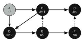
Constructing the depth first search tree
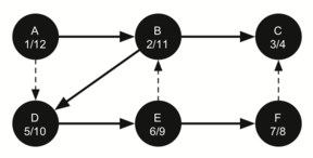
The starting and finishing times for each node display a property called the parenthesis property. This property means that all the children of a particular node in the depth first tree have a later discovery time and an earlier finish time than their parent.
9.5 Topological Sorting
கணினி விஞ்ஞானிகள் எதையும் ஒரு முனை-ஓரம் அடைவுப் பிரச்சனையாக மாற்ற முடியும் என்பதை நிரூபிக்க, ஒரு தொகுதி தட்டையான அப்பம் (pancakes) கிளறிவிடுவதில் உள்ள கடினமான பிரச்சனையை கருத்தில் கொள்வோம். செய்முறை மிகவும் எளிது: 1 முட்டை, 1 கோப்பை அப்பக் கலவை, 1 தேக்கரண்டி எண்ணெய், மற்றும் முக்கால் கோப்பை பால். அப்பத்தை தயாரிக்க நீங்கள் கட்டையை சூடாக்க வேண்டும், அனைத்து பொருட்களையும் ஒன்றாக கலந்து, கலவையை ஒரு சூடான தட்டில் வைக்கவும். அப்பங்கள் குமிழ ஆரம்பித்தவுடன் அவற்றைத் திருப்பி கீழே பொன்னிறமாகும் வரை சமைக்கவும். உங்கள் அப்பத்தை சாப்பிடுவதற்கு முன் நீங்கள் சில பாகங்களை சூடாக்க வேண்டும். முனை-ஓரம் அடைவாக இந்த செயல்முறை இங்கே:
The steps for making pancakes
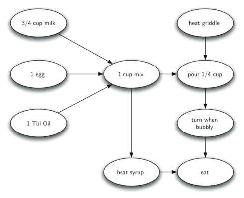
அப்பத்தை தயாரிப்பதில் உள்ள கடினமான விஷயம் முதலில் என்ன செய்வது என்று தெரிந்து கொள்வது. நீங்கள் கட்டையை சூடாக்குவதன் மூலம் அல்லது பான்கேக் கலவையில் ஏதேனும் பொருட்கள் சேர்ப்பதன் மூலம் தொடங்கலாம் என நீங்கள் மேலே பார்க்க முடியும். எங்கள் அப்பத்தை செய்ய தேவையான ஒவ்வொரு படிகளையும் நாம் செய்ய வேண்டிய துல்லியமான வரிசையை தீர்மானிக்க உதவுவதற்காக, topological sort எனப்படும் முனை-ஓரம் அடைவு வழிமுறைக்கு மாற்றுவோம்.
ஒரு இடவியல் வகைப்படுத்தப்பட்ட acyclic முனை-ஓரம் அடைவினை எடுத்து அதன் அனைத்து உச்சிகளின் நேரியல் வரிசையை உருவாக்குகிறது,அதாவது ஒரு முனை-ஓரம் அடைவு G ஆனது விளிம்புகள் v ,w ஐ கொண்டிருப்பின் உச்சி v ஆனது உச்சி w ஐ விட வரிசையில் முன்னதாக வரும்.இயங்கும் acyclic முனை-ஓரம் அடைவுகள் பல பயன்பாடுகளில் நிகழ்வுகளின் செயல்முறைப் படிகளைக் குறிக்க பயன்படுத்தப்படுகின்றன.அப்பத்தை தயாரிப்பது அப்படி ஒரு உதாரணமாகும். மற்ற எடுத்துக்காட்டுகளில் மென்பொருள் திட்ட அட்டவணைகள், தரவுத்தள வினவல்களை மேம்படுத்துவதற்கான முன்னுரிமை விளக்கப்படங்கள் மற்றும் அச்சு வார்ப்புருக்களின் பெருக்கல் ஆகியவை அடங்கும்.
இடவியல் வரிசை என்பது ஒரு ஆழமான முதல் தேடலின் எளிய ஆனால் பயனுள்ள தழுவலாகும். இடவியல் வகைக்கான வழிமுறை பின்வருமாறு:
- ஒவ்வொரு உச்சிகளின் முடிவடையும் நேரத்தை கணக்கிடுவதற்காக முதலில் வரைபடத்தில் ஒரு ஆழமான தேடலை செய்யவும்.
- உச்சிகளை முடிவடையும் நேரத்தின் குறைவடையும் வரிசையில் ஒரு பட்டியலில் சேமிக்கவும்.
- இடவியல் வரிசையின் விளைவாக வரிசைப்படுத்தப்பட்ட பட்டியலைத் திருப்பித் பதிலாக தரவும்.
மேலே காட்டப்பட்டுள்ள தட்டையான அப்பம் தயாரிக்கும் முனை-ஓரம் அடைவில் ஆழமான முதல் தேடுதல் மூலம் கட்டப்பட்ட ஆழத்தின் முதல் காட்டை கீழே உள்ள வரைபடம் காட்டுகிறது.
Result of Depth First Search on the Pancake Graph
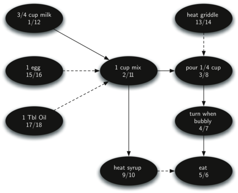
இறுதியாக, கீழே உள்ள முனை-ஓரம் அடைவு எங்கள் முனை-ஓரம் அடைவில் இடவியல் வரிசைமுறை வழிமுறையைப் பயன்படுத்துவதற்கான முடிவுகளைக் காட்டுகிறது. இப்போது அனைத்து தெளிவின்மையும் நீக்கப்பட்டு, தட்டையான அப்பம் செய்யும் படிகளைச் செய்ய வேண்டிய வரிசை எங்களுக்குத் தெரியும்.
Result of Topological Sort on Directed Acyclic Graph
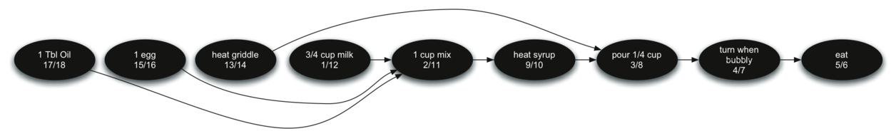
9.7 Shortest Path with Dijkstra’s Algorithm
When you surf the web, send an email, or log in to a laboratory computer from another location on campus a lot of work is going on behind the scenes to get the information on your computer transferred to another computer. The in-depth study of how information flows from one computer to another over the Internet is the primary topic for a class in computer networking. However, we will talk about how the Internet works just enough to understand another very important graph algorithm.
Overview of connectivity in the internet
The diagram above shows you a high-level overview of how communication on the Internet works. When you use your browser to request a web page from a server, the request must travel over your local area network and out onto the Internet through a router. The request travels over the Internet and eventually arrives at a router for the local area network where the server is located. The web page you requested then travels back through the same routers to get to your browser. Inside the cloud labeled “Internet” in the diagram are additional routers. The job of all of these routers is to work together to get your information from place to place. You can see there are many routers for yourself if your computer supports the traceroute command. The text below shows the output of running traceroute google.com on the author’s computer, which illustrates that there are 12 routers between him and the Google server responding to the request.
traceroute to google.com (216.58.192.46), 64 hops max, 52 byte packets
1 192.168.0.1 (192.168.0.1) 3.420 ms 1.133 ms 0.865 ms
2 gw-mosca207.static.monkeybrains.net (199.188.195.1) 14.678 ms 9.725 ms 6.752 ms
3 mosca.mosca-activspace.core.monkeybrains.net (172.17.18.58) 8.919 ms 8.277 ms 7.804 ms
4 lemon.lemon-mosca-10gb.core.monkeybrains.net (208.69.43.185) 6.724 ms 7.369 ms 6.701 ms
5 38.88.216.117 (38.88.216.117) 8.420 ms 11.860 ms 6.813 ms
6 be2682.ccr22.sfo01.atlas.cogentco.com (154.54.6.169) 7.392 ms 7.250 ms 8.241 ms
7 be2164.ccr21.sjc01.atlas.cogentco.com (154.54.28.34) 8.710 ms 8.301 ms 8.501 ms
8 be2000.ccr21.sjc03.atlas.cogentco.com (154.54.6.106) 9.072 ms
be2047.ccr21.sjc03.atlas.cogentco.com (154.54.5.114) 11.034 ms
be2000.ccr21.sjc03.atlas.cogentco.com (154.54.6.106) 10.243 ms
9 38.88.224.6 (38.88.224.6) 8.420 ms 10.637 ms 8.855 ms
10 209.85.249.5 (209.85.249.5) 9.142 ms 17.734 ms 12.211 ms
11 74.125.37.43 (74.125.37.43) 8.792 ms 9.290 ms 8.893 ms
12 nuq04s30-in-f14.1e100.net (216.58.192.46) 8.759 ms 8.705 ms 8.502 ms
Each router on the Internet is connected to one or more other routers. So if you run the traceroute command at different times of the day, you are likely to see that your information flows through different routers at different times. This is because there is a cost associated with each connection between a pair of routers that depends on the volume of traffic, the time of day, and many other factors. By this time it will not surprise you to learn that we can represent the network of routers as a graph with weighted edges.
Connections and weights between routers in the internet
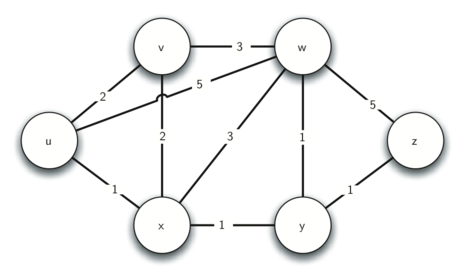
Above we show a small example of a weighted graph that represents the interconnection of routers in the Internet. The problem that we want to solve is to find the path with the smallest total weight along which to route any given message. This problem should sound familiar because it is similar to the problem we solved using a breadth first search, except that here we are concerned with the total weight of the path rather than the number of hops in the path. It should be noted that if all the weights are equal, the problem is the same.
Dijkstra’s Algorithm
The algorithm we are going to use to determine the shortest path is called “Dijkstra’s algorithm.” Dijkstra’s algorithm is an iterative algorithm that provides us with the shortest path from one particular starting node to all other nodes in the graph. Again this is similar to the results of a breadth first search.
To keep track of the total cost from the start node to each destination we will make use of a distances dictionary which we will initialize to 0 for the start vertex, and infinity for the other vertices. Our algorithm will update these values until they represent the smallest weight path from the start to the vertex in question, at which point we will return the distances dictionary.
The algorithm iterates once for every vertex in the graph; however, the order that we iterate over the vertices is controlled by a priority queue. The value that is used to determine the order of the objects in the priority queue is the distance from our starting vertex. By using a priority queue, we ensure that as we explore one vertex after another, we are always exploring the one with the smallest distance.
The code for Dijkstra’s algorithm is shown below.
import heapq def calculate_distances(graph, starting_vertex): distances = {vertex: float('infinity') for vertex in graph} distances[starting_vertex] = 0 pq = [(0, starting_vertex)] while len(pq) > 0: current_distance, current_vertex = heapq.heappop(pq) # Nodes can get added to the priority queue multiple times. We only # process a vertex the first time we remove it from the priority queue. if current_distance > distances[current_vertex]: continue for neighbor, weight in graph[current_vertex].items(): distance = current_distance + weight # Only consider this new path if it's better than any path we've # already found. if distance < distances[neighbor]: distances[neighbor] = distance heapq.heappush(pq, (distance, neighbor)) return distances example_graph = { 'U': {'V': 2, 'W': 5, 'X': 1}, 'V': {'U': 2, 'X': 2, 'W': 3}, 'W': {'V': 3, 'U': 5, 'X': 3, 'Y': 1, 'Z': 5}, 'X': {'U': 1, 'V': 2, 'W': 3, 'Y': 1}, 'Y': {'X': 1, 'W': 1, 'Z': 1}, 'Z': {'W': 5, 'Y': 1}, } print(calculate_distances(example_graph, 'X')) # => {'U': 1, 'W': 2, 'V': 2, 'Y': 1, 'X': 0, 'Z': 2} |
Dijkstra’s algorithm uses a priority queue, which we introduced in the trees chapter and which we achieve here using Python’s heapq module.
The entries in our priority queue are tuples of (distance, vertex) which allows us to maintain a queue of vertices sorted by distance.
When the distance to a vertex that is already in the queue is reduced, we wish to update the distance and thereby give it a different priority. We accomplish this by just adding another entry to the priority queue for the same vertex. (We also include a check after removing an entry from the priority queue, in order to make sure that we only process each vertex once.)
Let’s walk through an application of Dijkstra’s algorithm one vertex at a time using the following sequence of diagrams as our guide. We begin with the vertex uuu. The three vertices adjacent to uuu are v,w,v,w,v,w, and x. Since the initial distances to v,w,v,w,v,w, and x are all initialized to infinity, the new costs to get to them through the start node are all their direct costs. So we update the costs to each of these three nodes. The state of the algorithm is:
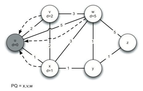
In the next iteration of the while loop we examine the vertices that are adjacent to u. The vertex x is next because it has the lowest overall cost and therefore will be the first entry removed from the priority queue. At x we look at its neighbors u,v,w and y. For each neighboring vertex we check to see if the distance to that vertex through x is smaller than the previously known distance. Obviously this is the case for y since its distance was infinity. It is not the case for u or v since their distances are 0 and 2 respectively. However, we now learn that the distance to w is smaller if we go through x than from u directly to w. Since that is the case we update w with a new distance and add another entry to the priority queue. The state of the algorithm is now:
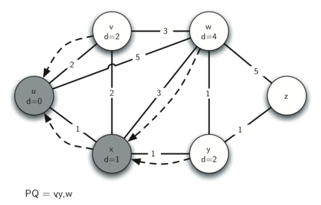
The next step is to look at the vertices neighboring v (below). This step results in no changes to the graph, so we move on to node y.
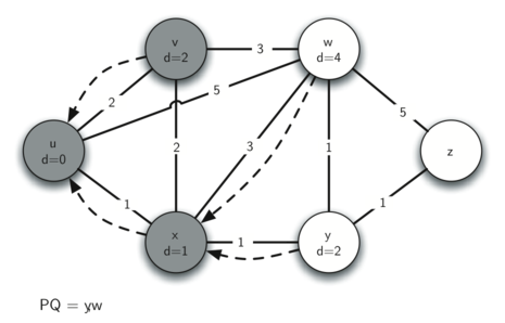
At node yyy (below) we discover that it is cheaper to get to both w and z, so we adjust the distances accordingly.
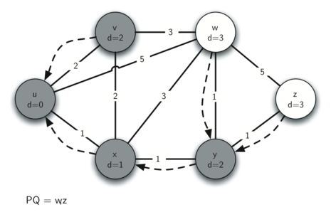
Finally we check nodes w and z. However, no additional changes are found and so the priority queue is empty and Dijkstra’s algorithm exits.
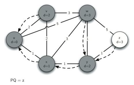
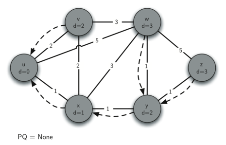
It is important to note that Dijkstra’s algorithm works only when the weights are all positive. You should convince yourself that if you introduced a negative weight on one of the edges to the graph that the algorithm would never exit.
We will note that to route messages through the Internet, other algorithms are used for finding the shortest path. One of the problems with using Dijkstra’s algorithm on the Internet is that you must have a complete representation of the graph in order for the algorithm to run. The implication of this is that every router has a complete map of all the routers in the Internet. In practice this is not the case and other variations of the algorithm allow each router to discover the graph as they go. One such algorithm that you may want to read about is called the “distance vector” routing algorithm.
Analysis of Dijkstra’s Algorithm
We will now consider the running time of Dijkstra’s algorithm.
Building the distances dictionary takes O(V) time since we add every vertex in the graph to the dictionary.
The while loop is executed once for every entry that gets added to the priority queue. An entry can only be added when we explore an edge, so there are at most O(E) iterations of the while loop.
The for loop is executed at most once for every vertex, since the current_distance > distances[current_vertex] check ensures that we only process a vertex once. The for loop iterates over outgoing edges, so among all iterations of the while loop, the body of the for loop executes at most O(E) times.
Finally, if we consider that each priority queue operation (adding or removing an entry) is O(logE), we conclude that the total running time is O(V+ElogE).
9.8 Strongly Connected Components
இந்த அத்தியாயத்தின் எஞ்சிய பகுதிகளுக்கு,சில பெரிய முனை-ஓரம் அடைவுகளில் நம் கவனத்தைத் திருப்புவோம். சில மேலதிக வழிமுறைகளைப் படிக்க நாம் பயன்படுத்தும் முனை-ஓரம் அடைவுகள் இணையத்தில் புரவலர்களுக்கும் இணையப் பக்கங்களுக்கிடையேயான இணைப்புகளுக்கும் இடையிலான இணைப்புகளால் உருவாக்கப்பட்ட முனை-ஓரம் அடைவுகள் ஆகும். நாங்கள் வலைப்பக்கங்களுடன் தொடங்குவோம்.
Google மற்றும் Bing போன்ற தேடுபொறிகளில் இணையத்தில் உள்ள பக்கங்கள் மிகப் பெரிய இயகங்கும் முனை-ஓரம் அடைவுகளளை உருவாக்குகின்றன.உலகளாவிய வலையை ஒரு முனை-ஓரம் அடைவாக மாற்ற, நாம் ஒரு பக்கத்தை ஒரு உச்சியாகக் கருதுவோம்,மேலும் பக்கத்தில் உள்ள மீத்தொடுப்புக்கள்(hyperlinks) ஒரு உச்சியை மற்றொரு உச்சியுடன் இணைக்கும் விளிம்புகளாகக் கருதுவோம்.கீழேயுள்ள விளக்கப்படம் லூதர் கல்லூரியின் கணினி அறிவியல் முகப்புப் பக்கத்தில் தொடங்கி, ஒரு பக்கத்திலிருந்து அடுத்த பக்கத்திற்கான இணைப்புகளைப் பின்பற்றுவதன் மூலம் உருவாக்கப்பட்ட முனை-ஓரம் அடைவின் மிகச் சிறிய பகுதியைக் காட்டுகிறது.நிச்சயமாக, இந்த முனை-ஓரம் அடைவு மிகப்பெரியதாக இருக்கலாம், எனவே கல்லூரியின் கணினி அறிவியல் முகப்புப் பக்கத்திலிருந்து 10 இணைப்புகளுக்கு மேல் இல்லாத வலைத்தளங்களுக்கு நாங்கள் அதை மட்டுப்படுத்தியுள்ளோம்.
The graph produced by links from the luther computer science home page
If you study the graph above you might make some interesting observations. First you might notice that many of the other web sites on the graph are other Luther College web sites. Second, you might notice that there are several links to other colleges in Iowa. Third, you might notice that there are several links to other liberal arts colleges. You might conclude from this that there is some underlying structure to the web that clusters together web sites that are similar on some level.
ஒரு முனை-ஓரம் அடைவில் மிகவும் ஒன்றோடொன்று இணைக்கப்பட்ட உச்சிகளைக் கண்டறிய உதவும் ஒரு ஒரு முனை-ஓரம் அடைவு வழிமுறை வலுவாக இணைக்கப்பட்ட கூறுகளின்-(strongly connected components) - (SCC) வழிமுறை என்று அழைக்கப்படுகிறது.ஒரு முனை-ஓரம் அடைவு G இல் உச்சிகளின் பெரிய துணைத்தொகுப்பு C Ebg hcgghv V ஆகும்.அதாவது ஒவ்வொரு ஜோடி உச்சிகளுக்கும் v, w \ C யில் ஆகும்.இதில் v இலிருந்து w வரை ஒரு வழி உள்ளது.அதேபோல் w இலிருந்து v வரை இன்னொரு வழி உள்ளது.இதனை வலுவாக இணைக்கப்பட்ட கூறுகள் என முறையா வரையறை செய்யலாம். கீழே உள்ள விளக்கம் மூன்று வலுவாக இணைக்கப்பட்ட கூறுகளைக் கொண்ட எளிய முனை-ஓரம் அடைவினைக் காட்டுகிறது. வலுவாக இணைக்கப்பட்ட கூறுகள் வெவ்வேறு நிழல் பகுதிகளால் அடையாளம் காணப்படுகின்றன.
A directed graph with three strongly connected components
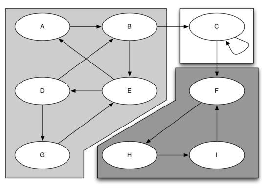
வலுவாக இணைக்கப்பட்ட கூறுகள் அடையாளம் காணப்பட்டவுடன், முனை-ஓரம் அடைவின் எளிமைப்படுத்தப்பட்ட பார்வையை ஒரு வலுவாக இணைக்கப்பட்ட ஒரு கூறுக்குள் உள்ள அனைத்து உச்சிகளையும் இணைத்து ஒற்றை பெரிய உச்சியில் சேர்க்கலாம். மேலே உள்ள முனை-ஓரம் அடைவின் எளிமைப்படுத்தப்பட்ட பதிப்பு கீழே காட்டப்பட்டுள்ளது.
The reduced graph
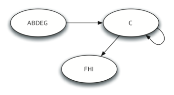
ஆழமான முதல் தேடலைப் பயன்படுத்துவதன் மூலம் நாம் மிகவும் சக்திவாய்ந்த மற்றும் திறமையான வழிமுறையை உருவாக்க முடியும் என்பதை மீண்டும் பார்ப்போம்.நாம் முக்கிய SCC வழிமுறையை கையாளும் முன் நாம் மற்றொரு வரையறையைப் பார்க்க வேண்டும். ஒரு முனை-ஓரம் அடைவின் எல்லா விளிம்புகளும் நேர்மாறல் ஆக மாற்றப்பட்டவுடன்,முனை-ஓரம் அடைவின் கால்ங்கள்-வரிகள் இடமாற்றம்(transpose) G என்பது முனை-ஓரம் அடைவின் GT ஆகும்.அதாவது, அசல் வரைபடத்தில் முனை A இலிருந்து முனை B க்கு இயக்கப்பட்ட விளிம்பு இருந்தால் GT ஆனது B முனையிலிருந்து முனை A வரை ஒரு விளிம்பைக் கொண்டிருக்கும்.கீழே உள்ள முனை-ஓரம் அடைவுகளானது ஒரு எளிய முனை-ஓரம் அடைவு மற்றும் அதன் இடமாற்றத்தைக் காட்டுகின்றன.
A graph G
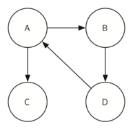
The transpose of G
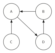
மேலே உள்ள முனை-ஓரம் அடைவுகள் வலுவாக இணைக்கப்பட்ட இரண்டு கூறுகளைக் கொண்டிருப்பதைக் கவனியுங்கள்.
ஒரு முனை-ஓரம் அடைவிற்கான வலுவாக இணைக்கப்பட்ட கூறுகளை கணக்கிடுவதற்கான வழிமுறையை நாம் இப்போது விவரிக்கலாம்.
- ஒவ்வொரு உச்சியின் முடிவடையும் நேரத்தைக் கணக்கிட G வரைபடத்தை முதலில் ஆழமாகத் தேடுங்கள்.
- GT ஐ கணக்கிடல்.
- முனை-ஓரம் அடைவினை GT ஆல் முதலில் ஆழமாகத் தேடுங்கள் ஆனால் பிரதானமாக மீள்செய்தலானது உச்சிகளின் முடிவடையும் நேரத்தின் குறைவடையும் வரிசையில் ஒவ்வொரு உச்சியையும் ஆராய்கிறது.
- படி 3 இல் கணக்கிடப்பட்ட காட்டில் உள்ள ஒவ்வொரு மரமும் வலுவாக இணைக்கப்பட்ட கூறு ஆகும். வெளியீடு செய்யும் உச்சிகளின் Id கள் காட்டிலுள்ள ஒவ்வொரு மரத்திலுமுள்ள ஒவ்வொரு உச்சிகளையும் கூறுகளில் அடையாளம் காண உதவும்.
வலுவாக இணைக்கப்பட்ட மூன்று கூறுகளுடன் மேலே உள்ள எடுத்துக்காட்டு முனை-ஓரம் அடைவில்,மேலே விவரிக்கப்பட்ட படிகளின் செயல்பாட்டைக் கண்டறியலாம். அசல் முனை-ஓரம் அடைவிற்காக கணக்கிடப்பட்ட தொடக்க மற்றும் இறுதி நேரங்கள் இங்கே:
Finishing times for the original graph G
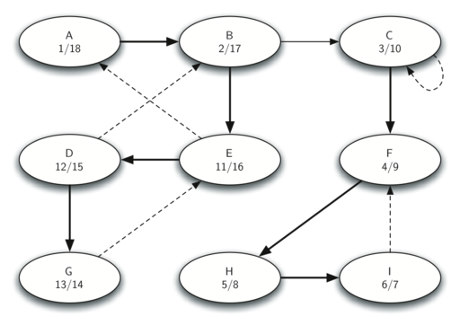
இடமாற்றப்பட்ட முனை-ஓரம் அடைவில் கணக்கிடப்பட்ட தொடக்க மற்றும் நிறைவு நேரங்கள் இங்கே.
Finishing times for the transpose of G
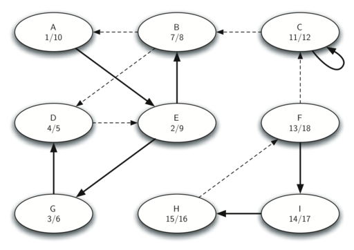
இறுதியாக, கீழே உள்ள விளக்கம் வலுவாக இணைக்கப்பட்ட கூறு வழிமுறையின் படி 3 இல் தயாரிக்கப்பட்ட மூன்று மரங்களின் காட்டை காட்டுகிறது. SCC வழிமுறைகளுக்கான பைதான் நிரலை நாங்கள் உங்களுக்கு வழங்கவில்லை என்பதை நீங்கள் கவனிப்பீர்கள், இந்த நிகழ்ச்சியை ஒரு பயிற்சியாக செய்வதற்கு விட்டுவிடுகிறோம்.
Strongly connected components
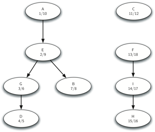
9.9 Prim’s Spanning Tree Algorithm
எங்கள் கடைசி முனை-ஓரம் அடைவு வழிமுறைக்கு , ஆன்லைன் விளையாட்டின் வடிவமைப்பாளர்கள் மற்றும் இணைய வானொலி வழங்குநர்கள் எதிர்கொள்கின்ற ஒரு சிக்கலைக் கருத்தில் கொள்வோம். சிக்கல் என்னவென்றால் செவிமடுத்துக்கொண்டிருக்கும் ஒவ்வொருவருக்கும் ஒரு தகவலை திறம்பட கொண்டுசேர்க்க வேண்டும்.இது இணைய விளையாட்டில் மிக முக்கியமானது ஏனென்றால் விளையாட்டில் ஈடுபடும் ஒருவருக்கு மற்றைய வீரர்களின் சமீபத்திய நிலைகள் தெரிய வேண்டும்.இது இணைய வானொலிக்கும் முக்கியமானது ஏனெனில் செவிமடுப்பவர்களுக்கு என்ன தேவையோ அதை வழங்க வேண்டும்.காரர்கள் ஒரு பாடலை கேட்டிட விரும்பினால் அதற்குரிய தகவல்களை வழங்க வேண்டும்.இந்த வரைபடம் ஒலிபரப்பு பிரச்சனையை விளக்குகிறது:
The broadcast problem
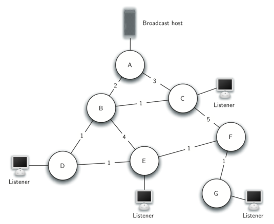
இந்த பிரச்சனைக்கு சில சிறந்த தீர்வுகள் உள்ளன, எனவே ஒலிபரப்பு பிரச்சனையை நன்கு புரிந்துகொள்ள உதவுவதற்கு முதலில் அவற்றைப் பார்ப்போம். இது முடிந்ததும் நாங்கள் முன்மொழியும் தீர்வைப் பாராட்ட இது உதவும். ஒலிபரப்பாளருக்கு கேட்போர் அனைவரும் பெற வேண்டிய சில தகவல்கள் உள்ளன. ஒலிபரப்பு நடத்துபவர் கேட்போர் அனைவரின் பட்டியலையும் ஒவ்வொருவருக்கும் தனிப்பட்ட செய்திகளை அனுப்புவதே எளிய தீர்வு. மேலே உள்ள வரைபடத்தில் ஒரு ஒலிபரப்பாளர் மற்றும் சில கேட்பவர்களுடன் ஒரு சிறிய இணைப்பைக் காட்டுகிறோம். இந்த முதல் அணுகுமுறையைப் பயன்படுத்தி, ஒவ்வொரு செய்தியின் நான்கு பிரதிகள் அனுப்பப்படும். இதற்க்கு குறைந்த செலவுடைய வழி பயன்படுத்தப்படுகிறது என்று வைத்துக்கொண்டால், ஒவ்வொரு திசைவியும் ஒரே செய்தியை எத்தனை முறை கையாளும் என்று பார்ப்போம்.
ஒலிபரப்பாளரிடமிருந்து அனைத்து செய்திகளும் திசைவி A வழியாக செல்கின்றன, எனவே A ஒவ்வொரு செய்தியின் நான்கு நகல்களையும் பார்க்கிறது. திசைவி C ஒவ்வொரு செய்தியின் ஒரு நகலை மட்டுமே அதன் கேட்பவருக்காகப் பார்க்கிறது. இருப்பினும், B மற்றும் D திசைவிகள் ஒவ்வொரு செய்தியின் மூன்று பிரதிகளையும் பார்க்கும், ஏனெனில் B மற்றும் D திசைவிகள் கேட்பவர்கள் 1,2 மற்றும் 3 இற்கு செலவு குறைந்த வழியில் உள்ளன.வானொலி ஒலிபரப்பிற்காக ஒலிபரப்பாளர் ஒவ்வொரு நொடியும் நூற்றுக்கணக்கான செய்திகளை அனுப்ப வேண்டும் என்று நீங்கள் கருதும் போது, அது கூடுதல் நெருக்கடியாகும்.
ஒலிபரப்பு செய்தியின் ஒரு பிரதியை ஒலி பரப்பு புரவலன்(host) அனுப்புவது மற்றும் திசைவிகள் விஷயங்களை வரிசைப்படுத்துவது ஒரு சிறந்த தீர்வாகும். இந்த சந்தர்ப்பத்தில் தீர்வின் உத்தி uncontrolled flooding என்று அழைக்கப்படும்.நிரம்பல் வழிதல் (flooding )உத்தி பின்வருமாறு செயல்படுகிறது.ஒவ்வொரு செய்தியும் உயிர்ப்புடன் இருக்கும் நேரத்துடன் தொடங்குகிறது (ttl) இதன் மதிப்பு ஒலிபரப்பு புரவலனுக்கும் அதன் தொலைதூர கேட்பவருக்கும் இடையில் உள்ள விளிம்புகளின் எண்ணிக்கையை விட அதிகமாகவோ அல்லது அதற்கு சமமாகவோ அமைக்கப்பட்டிருக்கும். ஒவ்வொரு திசைவியும் செய்தியின் நகலைப் பெற்று அதன் அண்டை திசைவிகள் அனைத்திற்கும் செய்தியை அனுப்புகிறது. செய்தி அனுப்பப்படும் போது Ttl இன் மதிப்பு குறைகிறது. Ttl மதிப்பு 0 ஐ அடையும் வரை ஒவ்வொரு திசைவியும் அதன் அனைத்து அண்டை திசைவிகளுக்கு செய்தியின் நகல்களை அனுப்புகிறது. uncontrolled flooding எங்கள் முதல் மூலோபாயத்தை விட பல தேவையற்ற செய்திகளை உருவாக்குகிறது என்பதை நீங்கள் காண முடியும்.
இந்த பிரச்சனைக்கு தீர்வு, குறைந்த எடை கொண்ட spanning tree ஐ உருவாக்குவதில் உள்ளது. முனை-ஓரம் அடைவு G = (V, E) இல் ஆகக்குறைந்த spanning tree T என்பதை வரையறுப்பதை பின்வருமாறு காட்டலாம்.T என்பது E இன் acyclic துணைக்குழு ஆகும், இது V யில் உள்ள அனைத்து முனைகளையும் இணைக்கிறது.T இல் உள்ள விளிம்புகளின் எடைகளின் தொகை குறைக்கப்படுகிறது.
கீழேயுள்ள முனை-ஓரம் அடைவுவானது ஒலிபரப்பு முனை-ஓரம் அடைவின் எளிமைப்படுத்தப்பட்ட பதிப்பைக் காட்டுகிறது மற்றும் முனை-ஓரம் அடைவிற்கான குறைந்தபட்ச spanning tree ஐ உருவாக்கும் விளிம்புகளை முன்னிலைப்படுத்துகிறது. இப்போது எங்கள் ஒலிபரப்பு சிக்கலை தீர்க்க, ஒலி பரப்பு புரவலன் ஒலி பரப்பு செய்தியின் ஒற்றை நகலை இணையத்திற்கு அனுப்புகிறது. ஒவ்வொரு திசைவியும் செய்தியை அனுப்பிய அண்டை திசைவியை தவிர்த்து, spanning tree இன் ஒரு பகுதியாக இருக்கும் எந்த அண்டை திசைவிக்கும் செய்தியை அனுப்புகிறது. இந்த எடுத்துக்காட்டில் A ஆனது B க்கு செய்தி அனுப்பப்படுகிறது.B ஆனது C மற்றும் D க்கு செய்தி அனுப்பப்படுகிறது.D ஆனது E க்கு செய்தி அனுப்பப்படுகிறது.E ஆனது F க்கு செய்தி அனுப்பப்படுகிறது.F ஆனது G க்கு செய்தி அனுப்பப்படுகிறது.எந்தவொரு திசைவியும் எந்த செய்தியின் ஒன்றுக்கு மேற்பட்ட நகல்களைப் பார்க்காது, ஆர்வமுள்ள அனைத்து கேட்பவர்களும் செய்தியின் நகலைப் பார்க்கிறார்கள்.
Minimum spanning tree for the broadcast graph
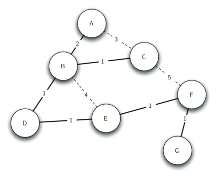
இந்த சிக்கலை தீர்க்க நாங்கள் பயன்படுத்தும் வழிமுறை Prim வழிமுறை என்று அழைக்கப்படுகிறது. Prim வழிமுறை “greedy algorithms” எனப்படும் வழிமுறைகளின் குடும்பத்தைச் சேர்ந்தது, ஏனென்றால் ஒவ்வொரு அடியிலும் நாம் செலவு குறைந்த அடுத்த படியை தேர்வு செய்வோம். இந்த சந்தர்ப்பத்தில் செலவுகுறைந்த அடுத்த கட்டம் என்பது குறைந்த எடையுடன் விளிம்பைப் பின்பற்றுவதாகும். எங்கள் கடைசி படி Prim வழிமுறையை உருவாக்குவதாகும்.
ஒரு spanning tree உருவாக்குவதற்கான அடிப்படை யோசனை பின்வருமாறு:
While T is not yet a spanning tree Find an edge that is safe to add to the tree Add the new edge to T |
பாதுகாப்பான ஒரு விளிம்பைக் கண்டுபிடிக்க வேண்டிய தந்திரம் நம்மை வழிநடத்தும் படியில் உள்ளது. spanning tree இல் இல்லாத ஒரு உச்சியை spanning tree இல் இருக்கும் ஒரு உச்சியுடன் இணைக்கும் எந்த விளிம்பும் பாதுகாப்பான விளிம்பு என நாங்கள் வரையறுக்கிறோம். எனவே இது சுழற்சிகள் இல்லாத ஒரு மரமாக இருப்பதை உறுதி செய்கிறது.
Prim வழிமுறையை செயல்படுத்த பைதான் குறியீடு கீழே காட்டப்பட்டுள்ளது. Prim வழிமுறை Dijkstra இன் வழிமுறையைப் போன்றது.அவர்கள் இரண்டும் வளர்ந்து வரும் முனை-ஓரம் அடைவில் சேர்க்க அடுத்த உச்சியைத் தேர்ந்தெடுக்கும் போது முன்னுரிமை வரிசையைப் பயன்படுத்துகின்றன.
from collections import defaultdict import heapq def create_spanning_tree(graph, starting_vertex): mst = defaultdict(set) visited = set([starting_vertex]) edges = [ (cost, starting_vertex, to) for to, cost in graph[starting_vertex].items() ] heapq.heapify(edges) while edges: cost, frm, to = heapq.heappop(edges) if to not in visited: visited.add(to) mst[frm].add(to) for to_next, cost in graph[to].items(): if to_next not in visited: heapq.heappush(edges, (cost, to, to_next)) return mst example_graph = { 'A': {'B': 2, 'C': 3}, 'B': {'A': 2, 'C': 1, 'D': 1, 'E': 4}, 'C': {'A': 3, 'B': 1, 'F': 5}, 'D': {'B': 1, 'E': 1}, 'E': {'B': 4, 'D': 1, 'F': 1}, 'F': {'C': 5, 'E': 1, 'G': 1}, 'G': {'F': 1}, } dict(create_spanning_tree(example_graph, 'A')) # {'A': set(['B']), # 'B': set(['C', 'D']), # 'D': set(['E']), # 'E': set(['F']), # 'F': set(['G'])} |
முனை-ஓரம் அடைவு பின்வரும் வரிசையில் எங்கள் மாதிரி மரத்தில் செயல்படும் வழிமுறையைக் காட்டுகிறது.நாம் உச்சி A இல் இருந்து ஆரம்பித்தால்,A அயலவர்களைப் பார்த்தால் , B மற்றும் C உச்சிகளுக்கு இடையேயான தூரத்தைப் புதுப்பிக்க முடியும்.ஏனென்றால் B மற்றும் C உச்சிகளுக்கு இடையேயான A இன் ஊடான தூரம் எல்லையற்றதை விடக் குறைவாகும்.நாம் B மற்றும் C யை சரியான வரிசையில் முன்னுரிமை வரிசையில் சேர்க்கலாம்.B மற்றும் C க்கான முன்னோடி இணைப்புகளை A. க்கு சுட்டிக்காட்டி அவற்றை மேம்படுத்தவும். நாம் இன்னும் spanning tree இல் B அல்லது C ஐ முறையாக சேர்க்கவில்லை என்பதை கவனத்தில் கொள்ள வேண்டும். முன்னுரிமை வரிசையில் இருந்து அகற்றப்படும் வரை ஒரு முனை spanning tree இன் ஒரு பகுதியாக கருதப்படவில்லை.
B க்கு மிகச்சிறிய தூரம் இருப்பதால் அடுத்ததாக B யைப் பார்ப்போம். B யின் அயலவர்களை ஆராய்ந்து பார்த்தால் D மற்றும் E புதுப்பிக்கப்படலாம். D மற்றும் E இரண்டும் புதிய தூர மதிப்புகளைப் பெறுகின்றன மற்றும் அவற்றின் முன்னோடி இணைப்புகள் புதுப்பிக்கப்படுகின்றன. முன்னுரிமை வரிசையில் அடுத்த முனைக்கு நகரும் போது நாம் காண்கிறோம். C க்கு அருகில் இருக்கும் ஒரே முனை C இன்னும் முன்னுரிமை வரிசையில் உள்ளது, எனவே நாம் F க்கு தூரத்தை புதுப்பித்து முன்னுரிமை வரிசையில் F இன் நிலையை சரிசெய்யலாம்.
இப்போது நாம் முனை D. க்கு அருகில் உள்ள உச்சிகளை ஆய்வு செய்கிறோம். நாம் E ஐ புதுப்பிக்கலாம் மற்றும் E இற்க்கான தூரத்தை 6 இலிருந்து 4 இற்கு குறைக்கலாம். இதைச் செய்யும்போது E இல் உள்ள முன்னோடி இணைப்பை D க்குச் சுட்டிக்காட்டி மாற்றுகிறோம்.spanning tree இல் ஒட்டப்பட்டது ஆனால் வேறு இடத்தில். மீதமுள்ள வழிமுறை நீங்கள் எதிர்பார்த்தபடி தொடர்கிறது, ஒவ்வொரு புதிய முனையையும் மரத்தில் சேர்க்கிறது
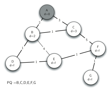
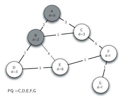
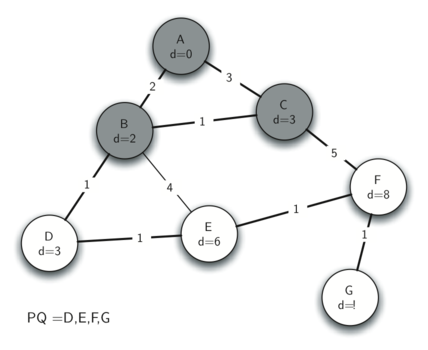
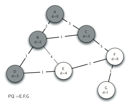
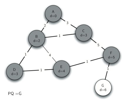
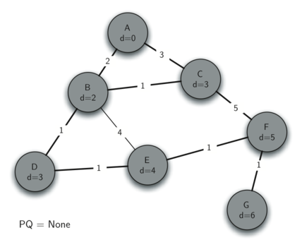
இணைப்பு - அ : அடிப்படடை தரவுவகைகள் - Fundamental Datatypes
பொதுவாக கணினி நிரலாக்கத்தில் (programming) பயான்படுத்தப்படும் அடிப்படை நிரலாக்கமொழி சார்ந்த கணினி தரவு வகைகள் இருக்கின்றன. இவையாவன, உதாரணம் C/C++-மொழியில், மற்றும் Python மொழியில் இந்த பட்டியலில் காணலாம்.

படம்: (set) கணம் - (தமிழ் விக்கிபீடியா சுட்டி)
தரவுவகை (datatype) | C/C++ மொழி | Python மொழி | விளக்கம் |
முழு எண்கள் (integer) | int, long, uint, … | int | முழு எண்கள் 0, 1, 2, 1024, 2048, ... |
தசம் எண்கள் (floating point) | float, double | float | 3.14159 போன்ற எண்கள் |
எழுத்து வகை (character) | char | chr | ‘அ' 'a’ போன்ற எழுத்துக்கள் |
சரம் (string) | char* | str | "சொல்" போன்ற சரங்கள் |
அணி (array/vector) | char[], int[],double[] #include<vector> std::vector<int> | list, [1,2,1,] | [“நாடு","கடந்த","நாடு"] போன்ற ஒரே வகையான தரவுகளைக் கொண்ட அணி; இவற்றில் உறுபடிகள் ஒன்று அல்லது பலமுறை இடம்பொறலாம். |
கணம் (set) | #include <set> std::set<int> | set, {1,2,..} | {“காவி”, “வெள்ளை”, “பச்சை”, “நீலம்”} போன்ற ஒரே வகையான தரவுகளைக் கொண்ட கணம்; இவற்றில் உறுபடிகள் ஒன்றுமுறை மட்டுமே இடம்பொறலாம். |
Glossary - கலைச்சொற்கள் அகராதி
|
|