How to Jupyter: A Brief Introduction to Jupyter Notebooks
Jupyter notebooks allow us to have a rich web-based interface to interactive python. Moreover, they allow for documenting and visualizing programming projects. They are widely used as a presentation tool in the data science community. The name "Jupyter" is a loose acronym for Julia, Python and R: the programming languages that the application originally targeted.
This document gives you a brief overview of how to read, interpret and use Jupyter notebooks. If you have any questions, please contact the CSCI 134 staff (cs134@cs.williams.edu).
Installing and Running Jupyter Notebooks
Step 1. Check if you already have the Jupyter notebook application installed by opening up the Terminal application[1] and running the following command. (If you followed the setup instructions for Windows/Mac on your machine, it should already be installed. All lab machines have the application installed as well.)
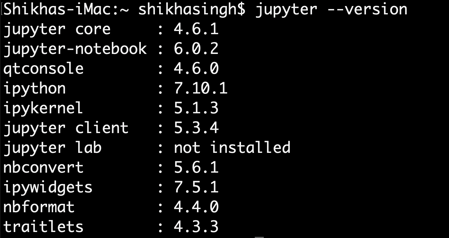
$ jupyter --version |
If you see information on all the components of the jupyter application (jupyter notebook, ipython, etc.) along with versions, then the application is already installed; move on to Step 2.
If you get a response that the command was not found, then you can install the application by running the following command (this assumes you already have pip3 installed). Do not try to manually install the individual components.
$ sudo pip3 install jupyterlab |
Step 2. Now we will learn how to open and run a Jupyter notebook. In the Terminal run the following command:
$ jupyter notebook |
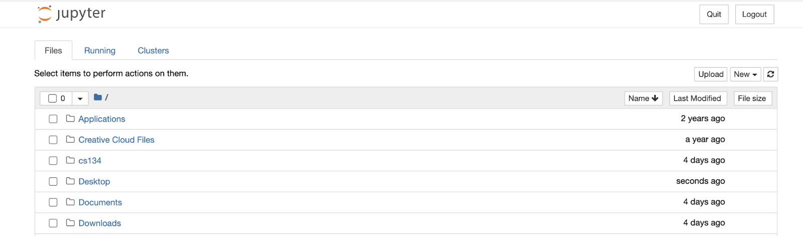
Your default browser window may open up automatically which shows the contents of your current directory.
If a browser doesn't open up, you should see instructions on how to open it in the Terminal:
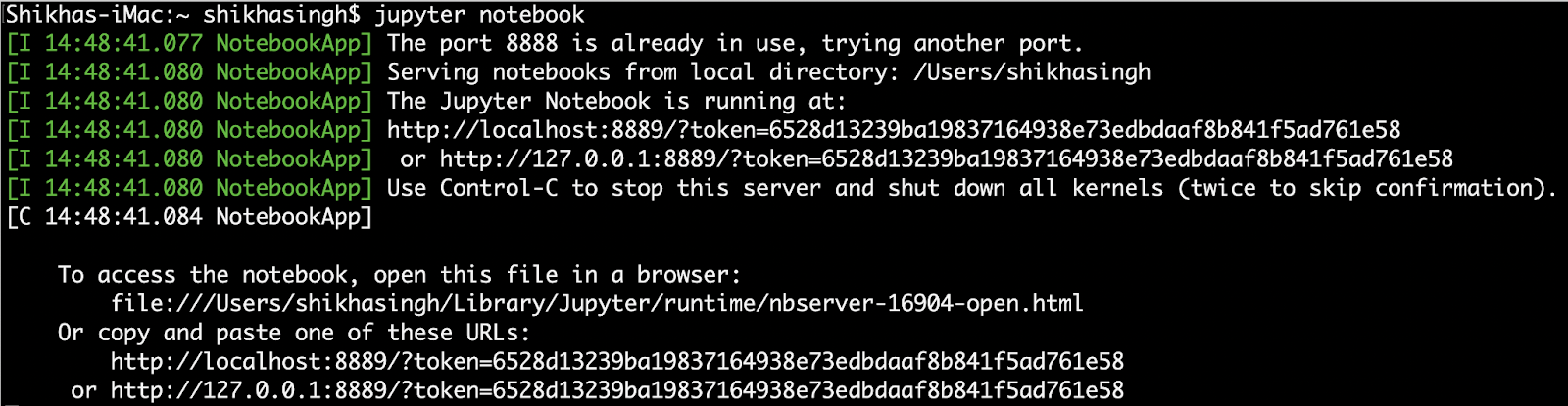
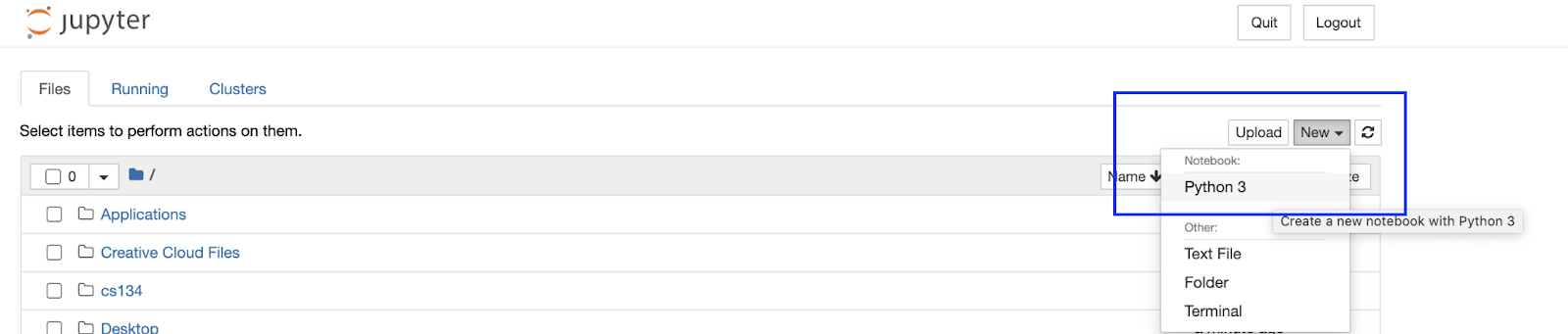
Copy and paste the URL in the instructions in your web browser to open the Jupyter application. You may create a new notebook by clicking on the "New" dropdown button on the top right, and choosing "Python3":
A new browser tab should open up with a blank input cell as shown:

You can now type in snippets of Python code in the "In[]" cell. E.g., suppose we want to know the length of the string 'Williams College'. We can type:

To run this code, select the cell (clicking on it will select it as seen by the blue highlight) and go to the Cell option in the top menu and choose "Run Cells". The keyboard shortcut to run cells is Shift+Enter/Return.
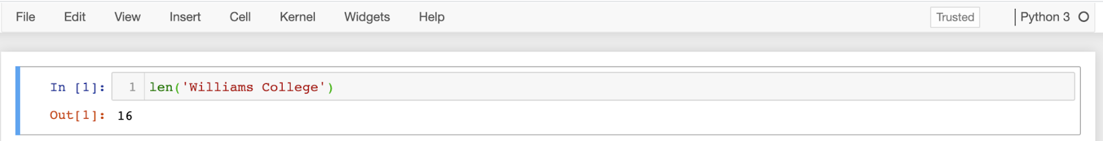
You should now see the output (in this case 16, which is the number of characters in the string 'Williams College') directly below with the label Out[1].
You can insert more cells by clicking on the "Insert" menu option and "Insert Cell below" and type in any other snippets of code you would like to test.
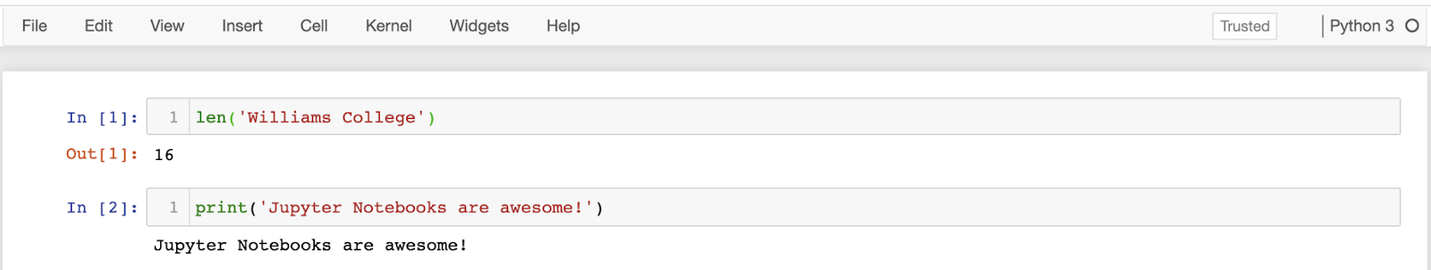
To understand the interface, note that typing a command in a In[] cell in a Jupyter notebook is similar to typing it in an interactive python session.
When we "run the cell," a number appears in the brackets to indicate that
- the command has been executed, and
- the number n indicates that it is the nth command executed in the current session.
In most cases, you can ignore this number. The Out[] cell of the notebook gives the resulting output.
Jupyter notebooks allow you to add rich notes along with examples: e.g., you can change the "Cell Type" (under the "Cell" menu option) to Markdown.
When you are done, you can save the notebook by selecting "File"-> "Save as" option. Closing the browser window does not exit out of the application on the Terminal. You can exit out of the Terminal by closing it, or by typing "Ctrl + C".
Downloading and Running a Notebook
We will be using Jupyter notebooks as a teaching aid in lectures, and posting the notebook on the course webpage (http://cs.williams.edu/~cs134/lectures.html).
You will find a sample Jupyter notebook under Resources , which we use here as an example. Jupyter notebook files have a .ipynb extension (which stands for interactive Python notebook).
Step 1. Go to the Resources page and download the Sample Notebook by right-clicking on the link and choosing Save As. Save the file to an easy-to-remember location.
Step 2. Use the directory interface on the Jupyter notebook application to navigate to this downloaded file, and click to open up the file. You can also navigate to the directory containing the file on the Terminal, and open by typing:
$ jupyter notebook lec_jupyter_intro.ipynb |
The notebook has a few prepopulated examples for you to try. You can execute each one-by-one by selecting the cell and running it ("Cell"->"Run Cells" or Shift+Enter/Return). If you would like to execute all of them at once, you can select "Cells->"Run All". Feel free to add notes or extra examples to this notebook (and to lecture notebooks in general).
Summary
Jupyter notebooks provide an enhanced way to use interactive python:
- they store code examples;
- code can be executed live very easily, and
- output is rendered in a rich format.
[1] We will use Terminal to mean the Terminal application on Mac and the Ubuntu application on Windows Subsystem for Linux. See the Mac and Windows setup documents for more details.