Road Map
Terminologies To know before start Neural Network and ML:
Imbalanced dataset, Training data, Validation Data, Testing Data, Voronoi cell 3D, Euclidean distance, Overfit, Underfit, Elongated,, Clustering, Quantisation , epoch (iteration),Mean-Deviation-Standard Deviation-VARIANCE, Square Root , Natural Log, Eigenvector and Eigenvalue , Distance matric, Gradient Descent and Linear Regression, Linear Equation on Graph, Linear Equation , Hot-Encoding, Independent Component Analysis (ICA), Natural Log, Covariance, Jacobian Matrix, Hyperplane Equation, Confusion Matrix, Metric space, Code Vector, Recall in ML, Regression in ML, Classifier machine learning, Feature Selection,Feature Extraction
Questions:
Why do we use linear algebra, matrices and vectors in machine learning algorithms?
Prerequisite:
Dr. Shabnam’s Math Lectures Learn by yourself
https://herts.instructure.com/courses/111121/modules/items/3637548
Lecture summary:
What is Vector ?
Length , direction and have reference point
https://herts.instructure.com/courses/111121/modules/items/3631897
Lecture summary:
- https://www.rapidtables.com/math/symbols/Basic_Math_Symbols.html
- https://simple.wikipedia.org/wiki/List_of_mathematical_symbols
- Linear algebra
- Trigonometry
- -> Unit circle https://www.youtube.com/watch?v=mhd9FXYdf4s&ab_channel=DennisDavis
- -> Sign Cos Function Wave https://www.youtube.com/watch?v=R6JCwzA8xX4&ab_channel=FredKong
- Derivative animation https://www.youtube.com/watch?v=53R2f5PLf7k&ab_channel=noureldinhassan
- Partial Derivatives
- https://www.youtube.com/watch?v=o93ILWVgqHI&ab_channel=JEESIMPLIFIED
- Vectors and matrices w.r.t ML
- https://www.youtube.com/watch?v=53R2f5PLf7k&ab_channel=BhautikiPlus
- joint probability distribution
Math offered by Hertfordshire University:
Skills that you’ll get.
Regression, classification, clustering, scikit-learn, and SciPy
Projects that you’ll do.
Cancer detection, predicting economic trends, predicting customer churn, recommendation engines.
Examples:
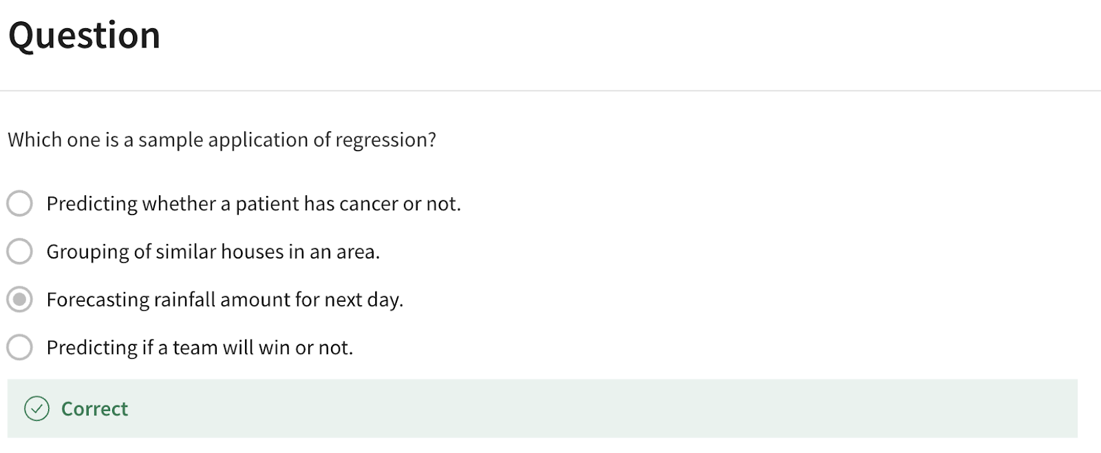
Regression/Estimation Technique:
- Predicts continuous values (e.g., house prices, CO2 emissions from a car).
Classification Technique:
- Predicts the class or category of a case (e.g., benign or malignant cells, customer churn).
Clustering Technique:
- Groups similar cases (e.g., patient similarity, customer segmentation).
Association Technique:
- Finds items or events that often co-occur (e.g., grocery items bought together by a customer).
Anomaly Detection:
- Identifies abnormal or unusual cases (e.g., credit card fraud detection).
Sequence Mining:
- Predicts the next event in a sequence (e.g., website click-stream).
Dimension Reduction:
- Reduces the size of data.
Recommendation Systems:
- Associates people's preferences with similar tastes and recommends new items (e.g., books, movies).
Introduction to Python for machine learning:
- NumPy, SciPy, Matplotlib, Pandas, SciKit Learn.
- NumPy: Efficient array operations.
- SciPy: Scientific computing and optimization.
- Matplotlib: Data visualization.
- Pandas: Data manipulation and analysis.
- SciKit Learn: Machine learning algorithms and tools.
Supervised learning and unsupervised learning:
Supervised learning: It's like teaching a machine learning model by giving it examples with labels. We show the model some data and tell it what the correct answer is. Then, the model learns from these examples and can make predictions on new, unseen data. For example, if we want to predict whether an email is spam or not, we can show the model many emails and tell it which ones are spam and which ones are not. The model learns from this labeled data and can predict if new emails are spam or not.
Unsupervised learning: It's like letting the machine learning model explore the data on its own. We don't give it labeled examples, but instead, it looks for patterns or structures in the data by itself. It tries to find similarities or groupings in the data without any prior knowledge. For example, if we have a dataset of customer purchases, the model can find groups of customers who buy similar products without us telling it what those groups are.
Supervised learning is used when we have labeled data and want to make predictions or classify things. Unsupervised learning is used when we want the model to find patterns or groupings in the data without any labels.
Regression is a method used to predict a continuous value based on other variables. It involves creating a model that relates a dependent variable (the value we want to predict) to one or more independent variables (the factors that influence the dependent variable). Regression can be simple (using one independent variable) or multiple (using multiple independent variables). It is used in various fields, such as sales forecasting, psychology, and predicting house prices. Regression helps us make predictions based on historical data and is a valuable tool for estimating outcomes.
For example, let's say we have data about cars, like their engine size, number of cylinders, and fuel consumption. We want to predict the amount of CO2 emissions a car will produce based on these factors. Regression helps us create a model that can estimate the CO2 emissions of a new car based on its engine size, cylinders, and other features.
There are two types of regression:
Simple regression, which uses one factor to predict the outcome, and
Multiple regression, which uses multiple factors.
Regression is used in many fields, like sales forecasting, psychology, and even predicting house prices. It's a useful tool for making predictions based on data.
Regression algorithms
- Ordinal regression .
- Poisson regression
- Fast forest quantile regression
- Linear, Polynomial, Lasso, Stepwise, Ridge regression
- Bayesian linear regression
- Neural network regression
- Decision forest regression
- Boosted decision tree regression
- KNN (K-nearest neighbors)
Principal Component Analysis:
Commonalities in ICA AND PCA
The key objective in PCA is to maximize the variance of the dataset in the lower-dimensional space. Mathematically, the variance retained after projecting the data onto the principal components is the sum of the corresponding eigenvalues. Selecting the top 𝑘 components typically involves choosing enough components to capture a large percentage of the total variance in the dataset.
Independent Component Analysis (ICA) and Principal Component Analysis (PCA) are both techniques used for dimensionality reduction and feature extraction, but they are based on different principles and assumptions. Here are some commonalities between ICA and PCA:
1. **Transformation Techniques**: Both ICA and PCA transform the original data into a new space.
2. **Linear Algebra**: Both methods use concepts and techniques from linear algebra, such as eigenvectors, eigenvalues, and matrix operations.
3. **Unsupervised Learning**: ICA and PCA are unsupervised learning techniques, which means they do not require labeled data to operate.
4. **Decorrelation of Components**: Both ICA and PCA seek to transform the original correlated variables into components that are linear combinations of the original variables and are uncorrelated with each other. PCA achieves this through orthogonal transformation, whereas ICA goes further to make the components statistically independent.
5. **Data Preprocessing Steps**: Both methods often begin with centering the data by subtracting the mean. PCA requires the data to be scaled or normalized, and while it's not always necessary for ICA, it can also benefit from whitening, which is a normalization that PCA inherently performs.
6. **Use in Signal Processing**: Both PCA and ICA are used in signal processing for noise reduction and signal separation.
7. **Dimensionality Reduction**: They can be used to reduce the dimensionality of the data by selecting a subset of components (principal components in PCA, independent components in ICA) to represent the original dataset.
8. **Covariance Matrix**: PCA involves the eigen-decomposition of the covariance matrix of the data to find the principal components. ICA can also involve covariance calculations, particularly during the whitening step, which precedes the independent component extraction.
Despite these commonalities, it's crucial to note that PCA and ICA are fundamentally different in their goals and results: PCA aims to capture the variance in the data with uncorrelated principal components, while ICA aims to uncover underlying factors that are statistically independent. PCA is a second-order method that only considers the variance (second-order moments), whereas ICA is a higher-order method that considers higher-order statistics to achieve independence of the components.
Sure, here's a list of both supervised and unsupervised learning algorithms:
**Supervised Learning Algorithms:**
1. Linear Regression
2. Logistic Regression
3. Support Vector Machines (SVM)
4. Decision Trees
5. Random Forests
6. Gradient Boosting Machines (GBM)
7. k-Nearest Neighbors (kNN)
8. Naive Bayes Classifier
9. Neural Networks (e.g., Multilayer Perceptrons)
10. Convolutional Neural Networks (CNN)
11. Recurrent Neural Networks (RNN)
12. Long Short-Term Memory networks (LSTM)
13. Extreme Gradient Boosting (XGBoost)
14. LightGBM
15. CatBoost
**Unsupervised Learning Algorithms:**
1. K-Means Clustering
2. Hierarchical Clustering
3. DBSCAN (Density-Based Spatial Clustering of Applications with Noise)
4. Gaussian Mixture Models (GMM)
5. Principal Component Analysis (PCA)
6. Independent Component Analysis (ICA)
7. t-distributed Stochastic Neighbor Embedding (t-SNE)
8. Self-Organizing Maps (SOM)
9. Autoencoders
10. Isolation Forest
11. Locally Linear Embedding (LLE)
12. Non-negative Matrix Factorization (NMF)
13. Spectral Clustering
14. Mean Shift Clustering
15. Adaptive Resonance Theory (ART)
These are some of the most commonly used algorithms in both supervised and unsupervised learning tasks across various domains.
Week 1- Introduction, Simple Competitive Learning and K-means
Machine Learning: Definitions
Machine learning involves computer algorithms that improve automatically through experience. The goal is for programs to perform tasks by learning from data rather than through explicit programming.
Supervised vs. Unsupervised Learning
Supervised Learning: Uses labeled data to predict outputs from inputs. It can be used for classification (categorical outputs) or regression (continuous outputs).
Unsupervised Learning: Works with unlabeled data to find inherent patterns or structures within the data, such as clusters or statistical structures.
Clustering
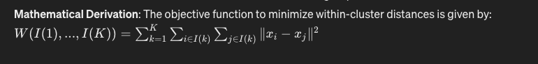
Clustering aims to group a set of objects in such a way that objects in the same group (a cluster) are more similar to each other than to those in other groups.
Mathematical Derivation:
W(I(1), ..., I(K)) = Σ from k=1 to K of Σ for i in I(k) of Σ for j in I(k) of ||x_i - x_j||²
K-Means Clustering
K-Means clustering tries to partition the dataset into K pre-defined distinct non-overlapping subgroups (clusters) where each data point belongs to only one group.
Mathematical Derivation:
Cluster Center: c_k = 1/|I(k)| Σ for i in I(k) of x_i
Sum of Squared Distances: S(I(1), ..., I(K)) = Σ from k=1 to K of Σ for i in I(k) of ||x_i - c_k||²

Simple Competitive Learning
This is a type of learning where fewer codevectors than data points are used to represent the data. The learning process iteratively adjusts the code vectors to minimise the quantization error.
Mathematical Derivation:
Quantization Error: E_quant = Σ from i=1 to n of min_k ||x_i - c_k||²
Codevector Update: c*_new = c* + λ (x - c*)

Online Resources:
Week 2 - Self-Organising Maps and Neural Gas
Codevectors / Vector Quantisation
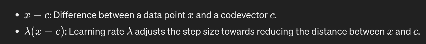
Code Vectors are elements in a vector space that represent data points. The goal is to find code vectors that minimise the distance to data points, providing a good representation of the data.
Mathematical Derivations:
x - c : Difference between a data point x and a codevector c.
λ(x - c) : Learning rate λ adjusts the step size towards reducing the distance between x and c.
Neural Gas
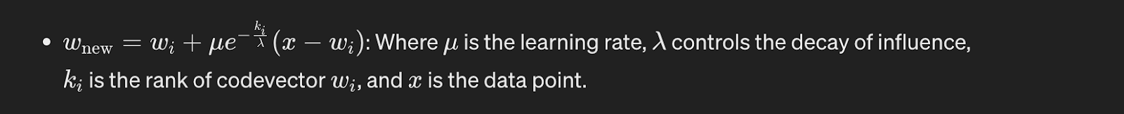
Neural Gas is an algorithm that models the topological structure of data using a flexible network of code vectors. It features adaptive learning where both the learning rate and the influence of each code vector diminish over time based on their rank determined by their distance to the current data point.
Neural Gas (NG) is a competitive learning algorithm used for clustering and topological organization of data in unsupervised learning scenarios. It is a variant of Self-Organizing Maps (SOMs) and was introduced by Thomas Martinetz and Klaus Schulten in 1991 as an alternative to the Kohonen Self-Organizing Map.
Neural Gas is particularly effective in scenarios where the data distribution is non-linear or contains clusters of varying densities. Unlike traditional clustering algorithms, Neural Gas does not require a predefined number of clusters. Instead, it adapts dynamically to the data distribution, allowing for flexible and adaptive clustering.
Here's an overview of how the Neural Gas algorithm works:
1. Initialization:
- Initialize a set of codebook vectors (or centroids) randomly or using a sampling strategy such as k-means initialization.
- Each codebook vector represents a prototype or cluster center in the feature space.
2. Adaptation:
- For each input data point, compute the distances between the input and all codebook vectors.
- Sort the codebook vectors based on their distances to the input data point.
- Update the codebook vectors' positions based on their ranking, with closer codebook vectors moving more towards the input data point.
- The update rule typically involves exponential decay, where closer codebook vectors receive larger updates.
3. Topology Preservation:
- Unlike traditional SOMs, Neural Gas employs a soft winner-take-all strategy, where multiple codebook vectors can be updated based on their distances to the input data point.
- This allows Neural Gas to preserve the topology of the input space more effectively, especially in scenarios with non-linear or high-dimensional data.
4. Learning Rate Adaptation:
- Neural Gas typically uses a decaying learning rate, where the learning rate decreases over time as the algorithm converges.
- This ensures that the algorithm converges smoothly and prevents abrupt changes in the codebook vectors' positions.
5. Convergence:
- The algorithm continues to update the codebook vectors iteratively until convergence criteria are met, such as a maximum number of iterations or a small change in the codebook vectors' positions.
Neural Gas has been applied in various domains, including pattern recognition, data clustering, and dimensionality reduction. Its ability to adapt to the data distribution and preserve the topology of the input space makes it a versatile and effective tool for unsupervised learning tasks.
Mathematical Derivations:
w_new = wi + μ e^(-ki/λ)(x - wi) : Where μ is the learning rate, λ controls the decay of influence, ki is the rank of codevector wi, and x is the data point.
Growing Neural Gas
This algorithm extends Neural Gas by dynamically adjusting the number of code vectors based on the local error observed in the data representation, adding new codevectors in regions with high error.
Mathematical Derivations:
w_new = w_old + μ0(x - w_old) : μ0 is the initial learning rate.
w_r = (w_q + w_f) / 2 : w_q and w_f are existing codevectors near high-error areas.

Self-Organising Maps (SOMs)
SOMs use a grid of codevectors and adaptively fit them to data by moving the codevectors towards data points while preserving the topological properties of the grid, useful for visualising and clustering high-dimensional data.
Mathematical Derivations:
w_new = wj + λ hij(x - wj) : Here λ is the learning rate, hij is a neighbourhood function based on the distance d(pi, pj) between the positions of codevectors in the grid.

Week 3 - Principal Component Analysis & Hierarchical Clustering
Co-leaner, Eigenvector, Eigenvalues,
Mean of already centered vector is ZERO
If the data is not centered, the first principal component might end up representing the mean of the data rather than variations around the mean.
PCA
- Project data onto new set of axis to reveal new pattern
- shifting the origin to the centroid of your data,
- squeezes and/or stretches the axes to make them equal in length, and
- rotates your axes into a new orientation.
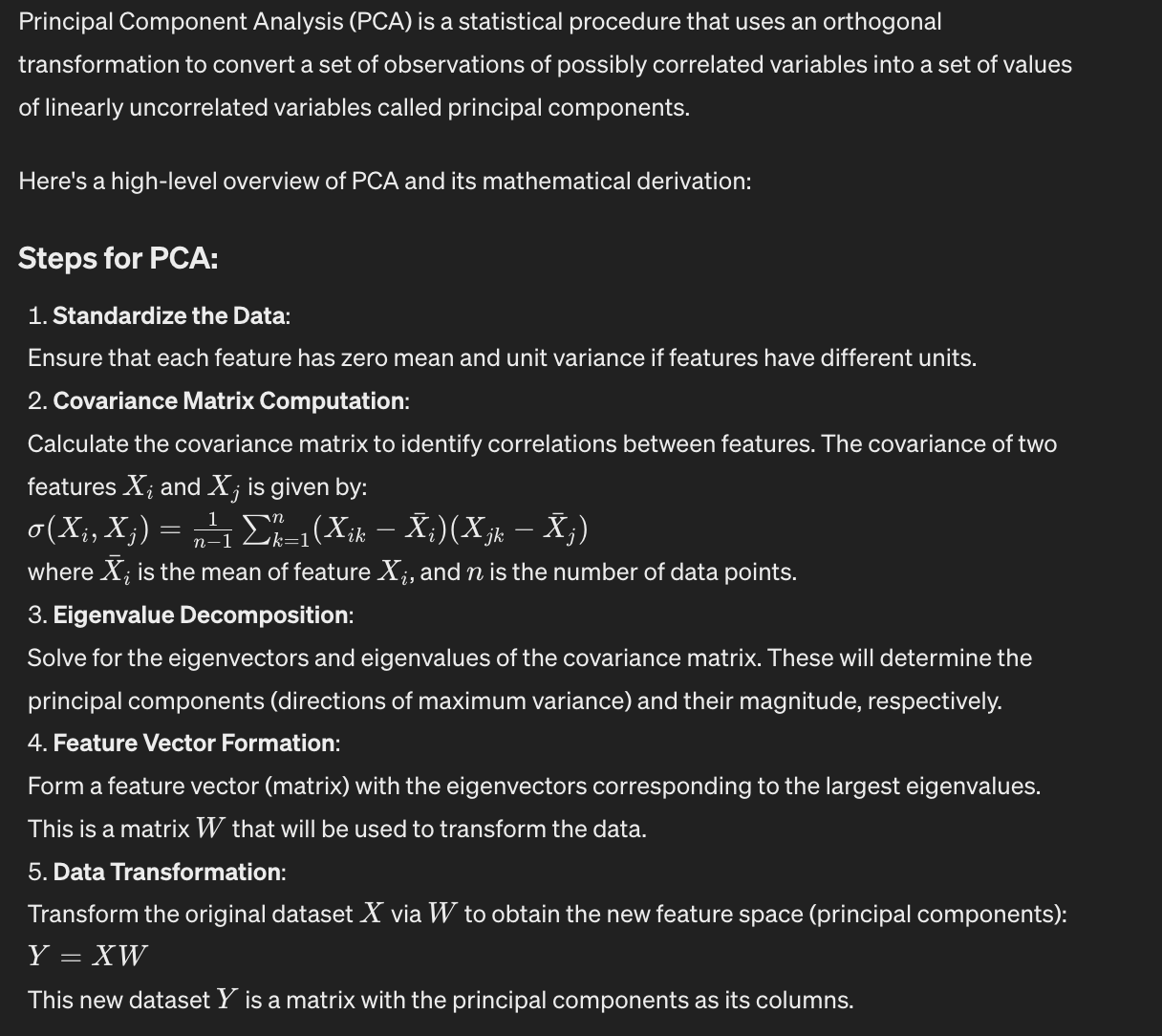
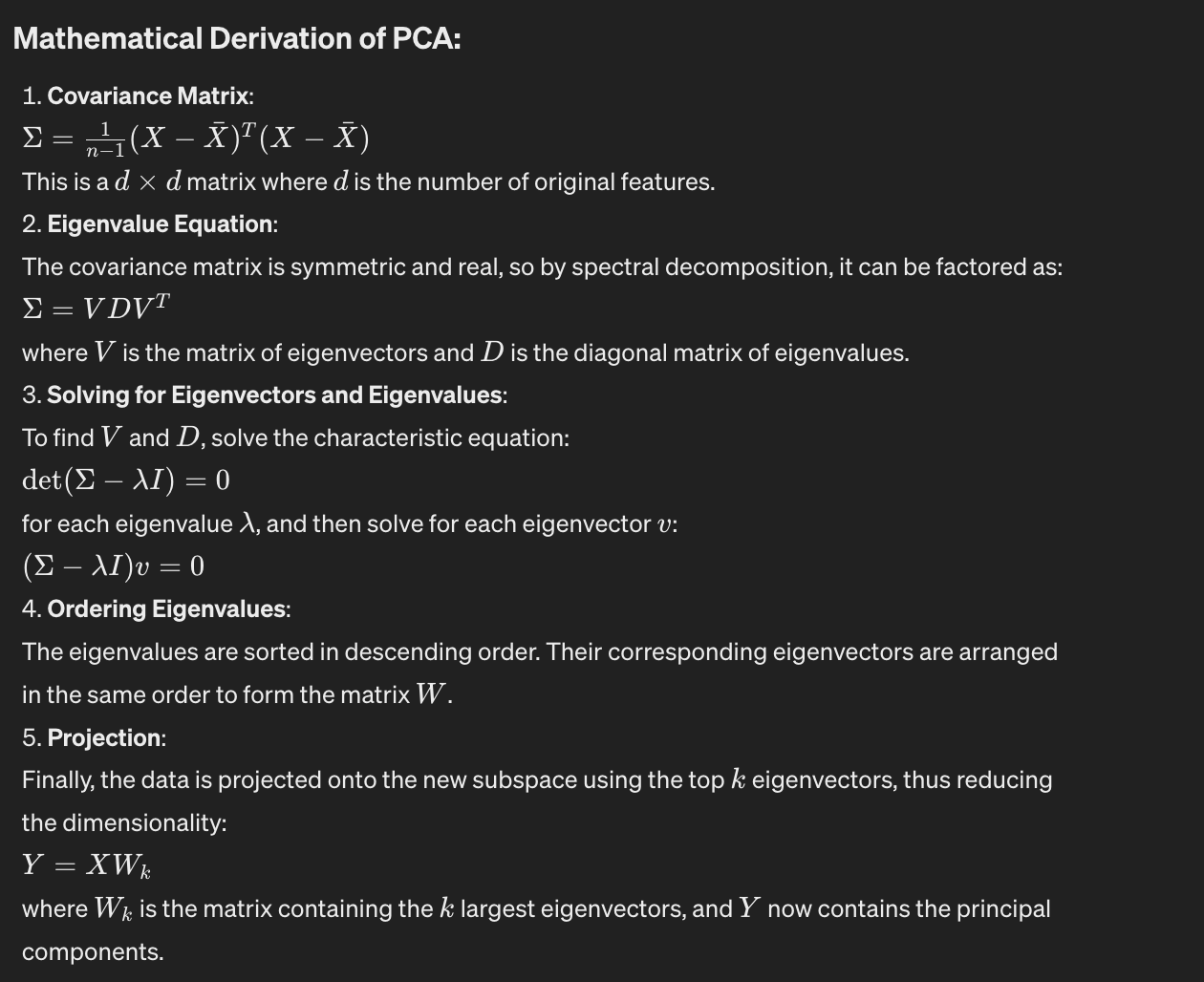
Principal Component Analysis (PCA) is a statistical procedure that uses an orthogonal transformation to convert a set of observations of possibly correlated variables into a set of values of linearly uncorrelated variables called principal components. Here's an overview of the steps involved in PCA, including the mathematical notations:
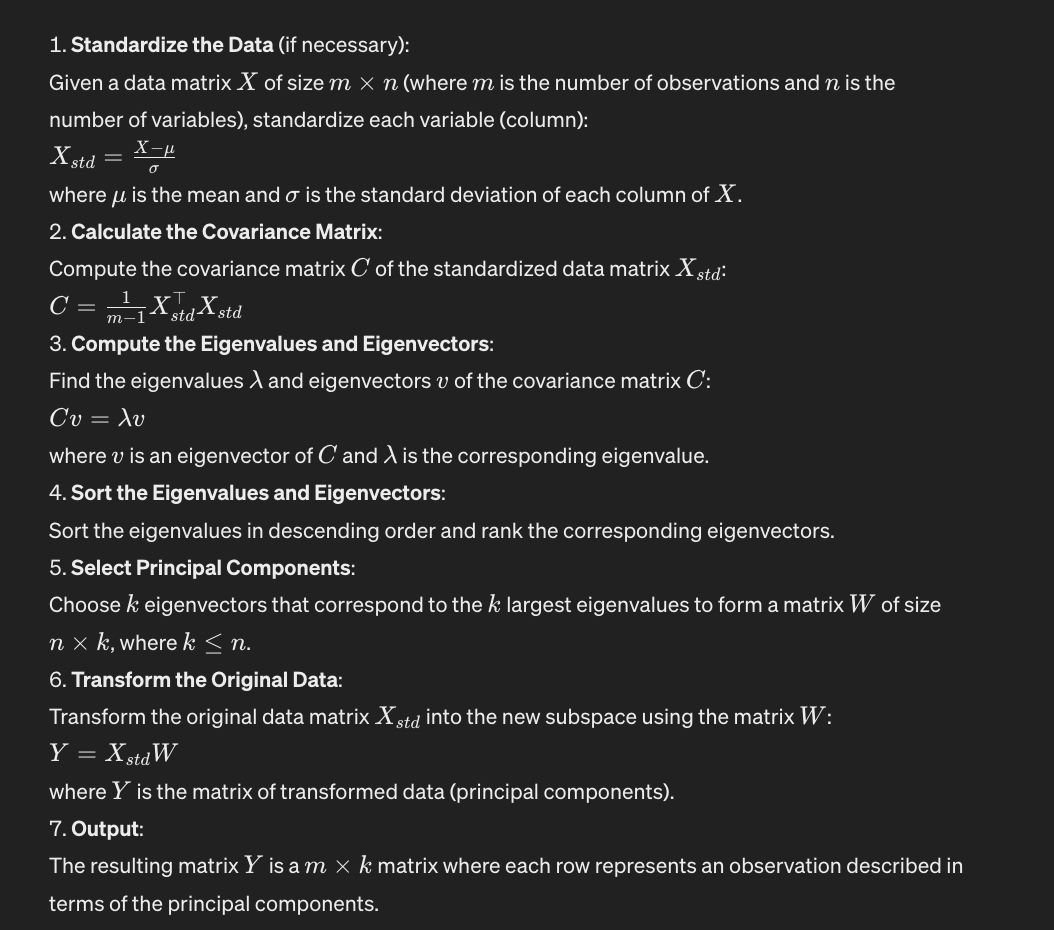
These steps summarize the process of PCA. The transformed data matrix \( Y \) now contains the principal components, and these components are uncorrelated. The first principal component accounts for the largest possible variance in the data, and each succeeding component has the highest variance possible under the constraint that it is orthogonal to the preceding components. The components are ordered so that \( \lambda_1 \geq \lambda_2 \geq ... \geq \lambda_n \), where \( \lambda_i \) is the eigenvalue corresponding to the \( i \)-th eigenvector.
Principal Component Analysis (PCA) is an unsupervised dimensionality reduction technique. It is used to simplify the complexity in high-dimensional data while retaining trends and patterns. In PCA, there is no use of class labels or any other form of supervision during the dimensionality reduction process. It works solely based on the input data, aiming to find the directions (principal components) that maximize the variance in the data.
However, PCA can also be used as a preprocessing step in supervised learning tasks. In such cases, PCA is applied to the input data to reduce its dimensionality, and then the reduced data is fed into a supervised learning algorithm. But the PCA itself does not require any supervision.
Hierarchical Clustering
Summary
◮ Heuristic method for data exploration.
◮ Visual impression of hierarchical structure.
◮ Use on samples of larger data sets.
◮ Operates on dissimilarity values.
◮ Similarity scores need to be transformed.
◮ Outputs a tree of nested clusters.
◮ Tree provides a partial ordering for items.
◮ Does not require interpolation.
◮ Requires dissimilarity matrix as input.
◮ Source data (e.g. data matrix) not required.
◮ Numerous combinations possible of
◮ dissimilarity measures,
◮ clustering criteria.
Recorded Video
https://herts.instructure.com/courses/111121/modules/items/3650201
Lecture Slide
Week 4 - Linear Models, K-Nearest Neighbors
Video Lecture by
https://www.youtube.com/watch?v=a22OPjS-4Lc&ab_channel=KrishNaik
Linear Regression in Machine Learning Explained in 5 Minutes
https://www.youtube.com/watch?v=YUPagM-OB_M&ab_channel=What%27sAIbyLouis-Fran%C3%A7oisBouchard
Simple Linear Regression at UH
Statistical technique used to model the relationship between two variables:
an independent variable (also known as the predictor variable) and
a dependent variable (also known as the response variable).
It assumes that there is a linear relationship between the two variables.
The goal of simple linear regression is to find the best-fitting line that represents the relationship between the variables. This line is determined by two parameters: the intercept (the point where the line crosses the y-axis) and the slope (the rate at which the line changes).
To perform simple linear regression, you need a dataset that includes observations of both the independent and dependent variables. By plotting the data points on a graph, you can visualize the relationship between the variables. The regression line is then fitted through the data points, aiming to minimize the distance between the line and the actual data points.
Once the regression line is established, it can be used to make predictions. Given a value for the independent variable, you can use the line to estimate the corresponding value of the dependent variable.
Simple linear regression is widely used in various fields, including economics, social sciences, and business, to analyze and predict the impact of one variable on another. It provides a straightforward and interpretable way to understand the relationship between two variables and make predictions based on that relationship.
Lecture Slide
Recorded Video
https://herts.instructure.com/courses/111121/modules/items/3659359
–
Gradient Descent Derivation:
https://www.youtube.com/watch?v=8zb9nsi8KzA&ab_channel=RANJIRAJ
–
Introduction to Regression
Regression is a method used in machine learning to predict a continuous value based on other variables. In simpler terms, it helps us estimate or guess a number based on some information we have. For example, let's say we have data about different cars, including their engine size, number of cylinders, and fuel consumption. Using regression, we can try to predict the amount of CO2 emissions a car will produce based on these factors.
How can regression be applied in sales forecasting? Can you provide an example?
Let's say we have a dataset that includes information about salespeople, such as their age, education level, and years of experience. We also have data on their total yearly sales. By using regression analysis, we can build a model that relates these independent variables (age, education, experience) to the dependent variable (total yearly sales).
Once the regression model is built, we can use it to predict the sales of a new salesperson based on their age, education, and experience. For instance, if we have a new salesperson who is 30 years old, has a bachelor's degree, and has 5 years of experience, we can input these values into the regression model and get an estimate of their expected total yearly sales.
This can be valuable for sales managers and organizations as it helps them forecast sales performance, allocate resources effectively, and make informed decisions about hiring, training, and incentivizing sales teams.
Real-life examples
Retail Industry: A retail company can use regression to predict the sales of a new product based on factors such as price, advertising expenditure, competitor prices, and customer demographics. By analyzing historical sales data and applying regression techniques, the company can estimate the potential demand for the new product and make informed decisions about production, inventory, and marketing strategies.
E-commerce: Online marketplaces can utilize regression to forecast sales based on variables like website traffic, customer behavior, promotional activities, and product attributes. By analyzing these factors and applying regression models, e-commerce platforms can estimate future sales volumes, optimize pricing strategies, and allocate resources effectively.
Hospitality Industry: Hotels and resorts can employ regression to predict room occupancy rates based on variables such as seasonality, local events, pricing, and customer reviews. By analyzing historical data and using regression techniques, hotel managers can forecast demand, optimize room rates, and plan staffing and inventory accordingly.
Consumer Goods: Companies in the consumer goods industry can use regression to forecast sales based on factors like consumer preferences, advertising expenditure, pricing, and economic indicators. By analyzing these variables and applying regression models, companies can estimate future sales volumes, plan production, and optimize marketing strategies.
Financial Services: Banks and financial institutions can utilize regression to forecast sales of financial products such as loans, credit cards, or insurance policies. By analyzing customer data, economic indicators, and other relevant variables, regression models can help predict customer demand, identify potential leads, and optimize sales strategies.
These are just a few examples of how regression can be applied in different industries. The specific variables and factors used in regression analysis may vary depending on the industry and context.
Simple Linear Regression
One independent variable is used to estimate a dependent variable. It also discusses the process of finding the best fit line for the data and how to calculate the parameters of the line.
Linear regression is useful because it is fast, doesn't require parameter tuning, and is easy to understand and interpret.
What are the key components of linear regression?
The key components of linear regression are:
Dependent variable: This is the variable that we want to predict or estimate. It is also known as the target variable.
Independent variable: This is the variable that we use to predict the dependent variable. It is also known as the predictor variable.
Simple linear regression: This is a type of linear regression where only one independent variable is used to estimate the dependent variable.
Multiple linear regression: This is a type of linear regression where more than one independent variable is used to estimate the dependent variable.
Coefficients: These are the parameters of the linear regression model. In simple linear regression, there are two coefficients: the intercept (theta 0) and the slope (theta 1). These coefficients determine the equation of the line that best fits the data.
Best fit line: This is the line that represents the relationship between the independent variable(s) and the dependent variable. It is determined by finding the values of the coefficients that minimize the mean squared error.
Mean squared error (MSE): This is a measure of how well the line fits the data. It is calculated by taking the average of the squared differences between the predicted values and the actual values of the dependent variable.
Prediction: Once the best fit line is determined, it can be used to make predictions for new data points by plugging in the values of the independent variable(s) into the equation of the line.
These components together form the foundation of linear regression, which is a powerful tool for predicting continuous values based on other variables.
How do you determine the best fit line in linear regression?
To determine the best fit line in linear regression, we aim to minimize the mean squared error (MSE) between the predicted values and the actual values of the dependent variable. Here's how it is done:
Start with a set of initial values for the coefficients (theta 0 and theta 1) of the line.
Calculate the predicted values of the dependent variable using the equation of the line.
Calculate the MSE by taking the average of the squared differences between the predicted values and the actual values of the dependent variable.
Adjust the values of the coefficients to minimize the MSE. This can be done using mathematical formulas or optimization algorithms.
Repeat steps 2-4 until the MSE is minimized or reaches a satisfactory level.
The values of the coefficients that minimize the MSE are considered the best fit line for the data.
It's important to note that in practice, most machine learning libraries and tools handle the process of finding the best fit line automatically, so you don't need to calculate the coefficients manually. However, understanding the concept of minimizing the MSE helps in interpreting and evaluating the results of linear regression models.
Model Evaluation in Regression Models
Feature Engineering: One-Hot Encoding
Hot encoding, also known as one-hot encoding, is a technique used in machine learning to represent categorical variables as binary vectors. Categorical variables are variables that take on a limited, fixed number of values (categories or levels), such as "red," "green," and "blue" for a variable representing colors.
Hot encoding works by creating a binary vector for each category in the categorical variable. Each vector has the same length as the number of categories, and all elements are set to zero except for the element corresponding to the category, which is set to one.
For example, suppose we have a categorical variable "colour" with three categories: red, green, and blue. Using hot encoding, we represent each category as follows:
- Red: [1, 0, 0]
- Green: [0, 1, 0]
- Blue: [0, 0, 1]
In this representation, each category is uniquely represented by a binary vector, and there is no inherent order or relationship between the categories. Hot encoding allows machine learning algorithms to effectively handle categorical variables as input features, as many machine learning algorithms require numerical input data.
Hot encoding is commonly used in tasks such as classification, where categorical variables need to be converted into a format that can be processed by machine learning models. It is important to note that hot encoding increases the dimensionality of the feature space, which may lead to computational challenges in cases of high cardinality categorical variables.
–
What is Generalisation ?
Generalisation in machine learning refers to the ability of a trained model to perform well on unseen data. In other words, a model that has generalised well has learned to capture the underlying patterns or relationships in the training data and can accurately make predictions on new, unseen examples from the same distribution.
The goal of training a machine learning model is not only to minimise the error on the training data but also to ensure that the model can generalise to new, previously unseen data points. Generalisation is essential because the ultimate aim of machine learning is to build models that can make accurate predictions on real-world data that the model has not encountered during training.
Achieving good generalisation requires balancing the model's complexity with the amount and quality of the training data. Overly complex models may overfit the training data and fail to generalise well to new data, while overly simple models may underfit the training data and also perform poorly on new data. Techniques such as regularisation, cross-validation, and collecting more diverse training data can help improve generalisation performance.
In summary, generalisation is a critical aspect of machine learning, and it refers to the ability of a trained model to accurately predict outcomes on new, unseen data points from the same underlying distribution as the training data.
–
What are Interpolation and Extrapolation?
Interpolation: Predict from inputs within training data range.
Extrapolation: Predict from inputs outside training data range
Interpolation and extrapolation are two different techniques used in predictive modelling:
1. Interpolation:
- Interpolation involves predicting outcomes for inputs that fall within the range of the training data.
- The model uses the patterns and relationships learned from the training data to make predictions for inputs that are similar to those it has seen before.
- Interpolation is the primary focus of most predictive modelling tasks, as it involves making predictions within the known range of the data.
2. Extrapolation:
- Extrapolation involves predicting outcomes for inputs that fall outside the range of the training data.
- This requires the model to extend or extrapolate the learned patterns and relationships beyond the range of the training data.
- Extrapolation can be challenging and risky because the model is making predictions based on assumptions about the behaviour of the data beyond what it has seen, which may not always hold true.
- Extrapolation should be approached with caution, and models should be validated to ensure their predictions are reliable and accurate, especially when extrapolating into unfamiliar regions of the input space.
In summary, interpolation involves predicting within the known range of the data, while extrapolation involves predicting outside this range, which can be more uncertain and requires careful consideration and validation.
What are null models?
Model that makes predictions using no information about the data or the features.
In machine learning, a null model is a simple model or benchmark that makes predictions based only on the most frequent outcomes, without regard to the input features. It's used as a baseline to compare the performance of more sophisticated models.
Example: In a dataset of emails classified as "spam" (20%) and "not spam" (80%), a null model would predict every email as "not spam" since that's the majority class. Despite ignoring the content of the emails, this null model would achieve 80% accuracy simply because "not spam" is the most common outcome.
Week 5 - Support Vector Machines, Classifier Performance
Lecture side
https://herts.instructure.com/courses/111121/files/8398193?wrap=1
Lecture Recording
https://herts.instructure.com/courses/111121/modules/items/3670878
When
To determine whether a model is suffering from overfitting or underfitting, we typically rely on evaluating its performance on a separate validation dataset or through techniques such as cross-validation. Here's how we can diagnose each case:
1. **Overfitting:**
- Overfitting occurs when a model learns to capture noise and idiosyncrasies in the training data, leading to poor generalization to unseen data.
- Signs of overfitting include high performance on the training dataset but poor performance on the validation dataset.
- Other indicators of overfitting include excessively complex models with a large number of parameters relative to the size of the training data, or when the model shows high variance in its predictions across different subsets of the data.
2. **Underfitting:**
- Underfitting occurs when a model is too simple to capture the underlying patterns in the data, leading to poor performance on both the training and validation datasets.
- Signs of underfitting include low performance on both the training and validation datasets, or when the model shows high bias in its predictions, consistently missing important patterns or trends in the data.
- Underfit models may also be characterized by poor convergence during training, or when the model's performance plateaus at a suboptimal level.
To address overfitting and underfitting, we can take the following steps:
- **Regularization:** Introduce regularization techniques such as L1 or L2 regularization to penalize overly complex models and discourage overfitting.
- **Feature Selection/Engineering:** Choose or engineer relevant features that capture the underlying structure of the data without introducing unnecessary complexity.
- **Cross-Validation:** Use techniques such as k-fold cross-validation to assess model performance on multiple subsets of the data and obtain a more reliable estimate of generalization error.
- **Model Complexity:** Adjust the complexity of the model by adding or removing features, adjusting hyperparameters, or using simpler or more complex model architectures based on the observed performance on the validation dataset.
- **Ensemble Methods:** Combine multiple models (e.g., bagging, boosting, stacking) to reduce overfitting and improve generalization performance.
By carefully monitoring the performance of the model on both the training and validation datasets, we can diagnose and mitigate issues related to overfitting and underfitting to improve the overall performance and generalization of the model.
Week 6 - Gaussian Processes, Reproducible ML
Mock Test
Extra Resources:
Neural network parameters without padding and stride
[N - f + 1 x N - f + 1]
[(n + 2 x p - f ) / s + 1]
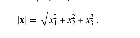
L^2-Norm (Euclidean Norm)
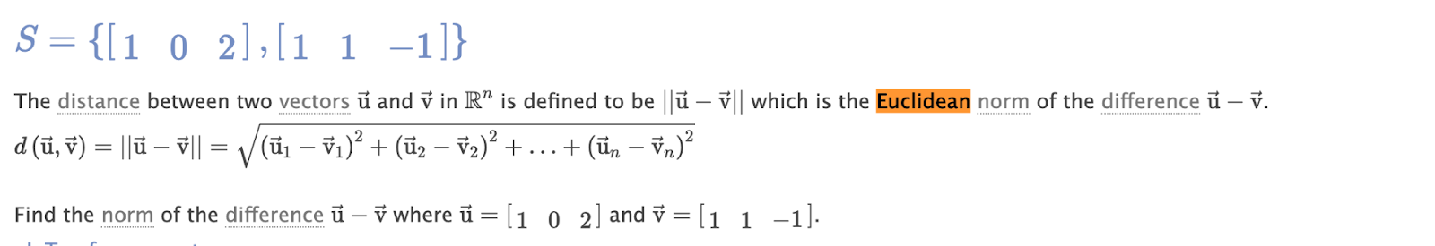
Euclidean Distance of Matrix
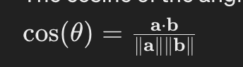
Cosine Angle
https://www.mathway.com/Algebra
https://mathworld.wolfram.com/Jacobian.html
Android: Maple Math App
Linear algebra graphical representation:
https://www.youtube.com/watch?v=4csuTO7UTMo&ab_channel=ZachStar
Jacobian:
https://www.youtube.com/watch?v=WUAQH2KQjMw&ab_channel=DigitalLearningHub-ImperialCollegeLondon
https://www.youtube.com/@thinking_neuron
Finding Local Maxima and Minima by Differentiation
https://www.youtube.com/watch?v=pvLj1s7SOtk&ab_channel=ProfessorDaveExplains
https://d2l.ai/chapter_convolutional-neural-networks/pooling.html
https://mathworld.wolfram.com/Plane.html
Probability Joint, Marginal, Bayes Theorem
https://www.youtube.com/watch?v=ndHDsvqmbuI&ab_channel=CampusX
Bayes Error:
https://www.youtube.com/watch?v=D0brk2U-WNU&ab_channel=TomVieringAI
https://www.youtube.com/watch?v=uoV1g3i9Qmw&ab_channel=MachineLearningTV
Feature Engineering: Ordinal, Label Encoding
https://www.youtube.com/watch?v=w2GglmYHfmM&ab_channel=CampusX
Hessian Normal Form
https://nccastaff.bournemouth.ac.uk/hncharif/MathsCGs/2010-2011/Analytic%20Geometry.pdf
https://www.deeplearningbook.org/
https://www.demogng.de/js/demogng.html?_3DV
In k-means clustering, we are interested in partitioning n observations into k clusters where each observation belongs to the cluster with the nearest mean. When k=2, we are splitting the data into two clusters.
For each data point, we have two choices: it can go to cluster 1 or cluster 2. However, since we don't consider the ordering of the clusters and all points cannot be in one cluster (otherwise it wouldn't be a partition), we need to adjust the count to avoid overcounting. We can consider the binary representations where each bit represents the cluster choice for each data point. For n data points, there are \(2^n\) possible combinations. However, this includes two invalid options where all data points are in either cluster 1 or cluster 2 (which are not partitions). Therefore, the correct number of ways to partition n items into 2 clusters is \(2^n - 2\), which is not listed in your options.
From the options provided, \(2^n - 1\) is the closest, but it only excludes one of the invalid options where all items are in the same cluster. The exact answer should be \(2^n - 2\), so if this is a question from a test or assignment, there might be a mistake in the provided options.
In the context of a vector quantization algorithm, the learning rate determines how much the codewords (or codevectors) are adjusted with each update during the training process. Increasing the learning rate typically makes the codewords adjust more rapidly to the data points. This can have several potential effects:
1. If the learning rate is increased slightly and is still within a reasonable range, it might help the codevectors to converge more quickly to a suitable representation of the data distribution, as each update makes a larger adjustment.
2. However, if the learning rate is too high, it can cause the algorithm to overshoot the optimal solution, potentially causing the codevectors to diverge or to oscillate around the optimal value without ever converging. This would mean that the area in which the codevectors move around after convergence increases, because they don't settle down to stable positions.
3. It will not directly cause the data points to move closer to the codevectors; rather, it affects how the codevectors move to better approximate the data points.
4. It doesn't necessarily cause the codevectors to converge more slowly unless the learning rate is so high that it causes divergence or oscillation, as mentioned in point 2.
Given these considerations, the most likely correct answer from the provided options is that the area in which the codevectors move around after convergence increases, assuming that "after convergence" is meant to refer to the behavior during the learning process rather than after it has properly converged. This would be a way of saying that the codevectors do not stabilize, which is a potential result of a too high learning rate. However, the wording of that option is somewhat ambiguous, as typically once convergence is reached, the vectors should not move much at all. If we interpret "after convergence" literally, as what happens once the algorithm has finished running, then none of the options are entirely correct.
Therefore, based on a generous interpretation of the options, the second option might be considered correct, but it would be advisable to seek clarification on the wording.
The Neural Gas algorithm is a type of vector quantization algorithm used for clustering and vector quantization that organizes the reference vectors (codewords) in a way similar to the Self-Organizing Map (SOM), but without a predefined grid structure. Let's examine the given statements one by one:
1. **The initial edge set contains all possible edges.**
- This statement is not typically true for the Neural Gas algorithm. The algorithm starts with no edges and incrementally builds a neighborhood graph by connecting nodes (neurons) based on their distances to the input signal. It does not start with a fully connected graph.
2. **Increasing the maximal edge age \( a_{max} \) results in a graph with more edges.**
- This statement is correct. In the Neural Gas algorithm, edges between nodes are aged and potentially removed if they become too old. If \( a_{max} \), the maximum allowed age for edges, is increased, edges will survive for longer, leading to a graph with more edges over time since fewer edges are removed due to aging.
3. **A codevector \( c \) will never be moved towards a data point \( d \) if there exists another data point \( d' \) such that \( ||d' - c|| < ||d - c|| \).**
- This statement is not accurate. In the Neural Gas algorithm, a codevector \( c \) is moved towards the data point \( d \) that is currently being considered, regardless of the existence of a closer data point \( d' \). The movement of \( c \) is based on its rank in terms of distance from the data point \( d \) being presented to the network, not the presence of other data points.
4. **The effective learning rate for each codevector depends on its rank, in terms of closeness to the currently selected data point.**
- This statement is correct. In the Neural Gas algorithm, when a data point is presented, the codevectors are ranked according to their distance from the data point, and the learning rate for updating each codevector is modulated based on this rank. Closer codevectors have a higher learning rate and hence move more towards the data point than those that are further away.
Based on these assessments, the correct statements about the Neural Gas algorithm are that increasing the maximal edge age \( a_{max} \) results in a graph with more edges, and the effective learning rate for each codevector depends on its rank, in terms of closeness to the currently selected data point.
Given the update rule of the Neural Gas algorithm:
\[ w_{i}^{new} = w_{i} + \mu \exp\left(-\frac{k_{i}}{\lambda}\right)(x - w_{i}) \]
Here's what each of the statements mean in the context of this formula:
1. **The amount of codevector movement decreases overall if λ is increased.**
- Correct. The variable λ in the denominator inside the exponential function acts as a smoothing factor for the rank-based learning rate modulation. As λ increases, the value of the exponential term decreases, especially for codevectors with higher rank numbers (less close to x), thus reducing the overall adjustment made to each codevector.
2. **In relative terms, the closest codevector would move by a larger amount if it were even closer to x.**
- This statement might be misleading as written. The relative movement is determined by the learning rate \( \mu \) and the rank \( k_{i} \), not by the current distance to \( x \). However, if \( k_{i} \) is lower (meaning that the codevector is closer in rank, not necessarily in Euclidean distance), then the movement is indeed larger because the exponential term would be larger. So if the statement is referring to rank as the measure of "closeness," then it is correct.
3. **The relative movement towards x is larger for codevectors closer to x.**
- Correct. For the closest codevector, \( k_{i} \) would be the smallest, making the exponential term larger, which in turn means that this codevector would have a larger adjustment towards \( x \) relative to codevectors that are further away in rank.
4. **In absolute terms, the most distant codevector would move by a larger amount if it were even further away from x.**
- Incorrect. The movement of each codevector is scaled by the exponential of the negative rank. Therefore, the further the codevector's rank, the smaller the exponential factor, and thus the smaller the movement towards \( x \). If a codevector's rank \( k_{i} \) were to increase because it is further away, its movement towards \( x \) would decrease, not increase.
So, the correct statements according to the update formula provided would be:
- The amount of codevector movement decreases overall if λ is increased.
- The relative movement towards x is larger for codevectors closer to x.
Let's evaluate the given statements about vector quantization:
1. **Features with a variance greater than one should be rescaled to unit variance, as that reduces quantization error.**
- Correct. Normalizing features to unit variance is a common preprocessing step in many data processing tasks, including vector quantization. It ensures that all features contribute equally to the quantization error and prevents features with larger variance from dominating the distance measures used in the quantization process.
2. **The learning rate should be set to a small value to prevent overfitting.**
- This statement is somewhat misleading in the context of vector quantization. The learning rate in vector quantization algorithms doesn't typically control overfitting in the same way it does in supervised learning models. In vector quantization, a learning rate that is too high can cause instability in the convergence of codevectors, while a rate that is too low can lead to slow convergence. Overfitting isn't usually a concern with vector quantization as it is an unsupervised learning algorithm, and the goal is to capture the distribution of the data.
3. **The training process generally aims to place codevectors close to data points, thereby minimizing quantization error.**
- Correct. The primary goal of vector quantization is to find a set of codevectors such that the average distortion or quantization error between the data points and their nearest codevectors is minimized. This means that the training process will adjust the codevectors to be as close as possible to the data points.
4. **The number of codevectors should be substantially smaller than the number of data points.**
- Correct. The idea of vector quantization is to represent the data with a smaller set of vectors (codevectors or centroids) to compress the dataset or reduce its dimensionality. If the number of codevectors were not substantially smaller than the number of data points, the benefits of quantization would be negated.
Based on these evaluations, the correct statements are:
- Features with a variance greater than one should be rescaled to unit variance, as that reduces quantization error.
- The training process generally aims to place codevectors close to data points, thereby minimizing quantization error.
- The number of codevectors should be substantially smaller than the number of data points.
Principal Component Analysis (PCA) is a statistical procedure that uses an orthogonal transformation to convert a set of observations of possibly correlated variables into a set of values of linearly uncorrelated variables called principal components. Here are the correct statements among the ones listed:
1. **Each principal component is orthogonal to all other principal components because the covariance matrix is symmetric.**
- Correct. PCA works by eigen decomposition of the data covariance matrix or singular value decomposition of the data matrix, both of which produce orthogonal (uncorrelated) eigenvectors that represent the principal components.
2. **The coordinate system of principal components is rotated relative to the original coordinate system, such that the amount of variance in the direction of the first principal component is maximised.**
- Correct. PCA rotates the coordinate system so that the greatest variance by any projection of the data comes to lie on the first axis (the first principal component), the second greatest variance on the second axis, and so on.
3. **The number of principal components is (at most) equal to the number of input features.**
- Correct. The maximum number of principal components you can get is equal to the number of input features or the number of observations, whichever is smaller. However, typically the number of observations is larger, so the number of input features sets the limit.
4. **Repeated application of PCA results in increasing the amount of variance in the direction of the first principal component.**
- Incorrect. Repeated application of PCA does not increase the amount of variance captured by the first principal component. The amount of variance captured by each principal component is determined by the data itself and PCA simply finds the directions (principal components) that capture this variance. Applying PCA multiple times does not change the underlying data or its variance distribution.
So, the first three statements are correct and the fourth one is incorrect.
In order for a function to be considered a valid distance metric in the strict mathematical sense, it must satisfy the following properties:
1. **Non-negativity**: The distance between any two points must be non-negative.
2. **Identity of indiscernibles**: The distance between any point and itself must be zero, and if the distance between two points is zero, they must be the same point.
3. **Symmetry**: The distance from point A to point B must be the same as the distance from point B to A.
4. **Triangle inequality**: The distance from point A to point C must be less than or equal to the distance from point A to point B plus the distance from point B to point C.
Let's analyze the provided functions according to these criteria:
`f1` function:
This function computes the Euclidean distance between two vectors. It satisfies all the properties of a valid distance metric.
`f2` function:
This function calls `f1`, but it incorrectly provides the same vector `x` for both parameters of `f1`, meaning it will always return zero. This does not satisfy the identity of indiscernibles because two different points could return a distance of zero, which shouldn't happen unless they are the same point.
`f3` function:
This function calculates the distance by comparing only the first half of vector `x` with the first half of vector `y`. This does not satisfy the identity of indiscernibles property because two vectors could be different in the second half but be considered zero distance apart by this function.
`f4` function:
This function appears to attempt a normalized distance, but it does so by dividing the dot product of `x` and `y` by the product of the distances of `x` to itself and `y` to itself. This does not satisfy the properties of a distance metric, particularly because the distance from a vector to itself should be zero (identity of indiscernibles), which would make the denominator zero and the result undefined.
Given these analyses, the correct statement is:
- `f1` is a valid distance.
Hierarchical clustering is a method of cluster analysis which seeks to build a hierarchy of clusters. The topology of the clustering tree (dendrogram) can be affected by the way distances are measured between the data points. Let's consider the given operations:
1. **Centering all features to zero mean.**
- This typically does not change the relative distances between data points, assuming the scaling of the features remains unchanged. Centering the data can make it easier to interpret, but it doesn't alter the topology of the tree in hierarchical clustering.
2. **Rotating the input data, e.g., from their original space into principal component space.**
- Rotating the data into principal component space changes the axes along which the data variance is measured but doesn't change the relative Euclidean distances between points. Therefore, if the distance metric used is the Euclidean distance, this operation should not change the topology of the hierarchical clustering tree.
3. **Using the L1 norm instead of the L2 norm to construct the distance matrix.**
- This can significantly change the topology of the hierarchical clustering tree. The L1 norm (Manhattan distance) and L2 norm (Euclidean distance) measure distances differently. The L1 norm can change the distances between points, especially in higher dimensions, which would result in a different dendrogram.
4. **Scaling all features to unit variance.**
- Scaling features to unit variance changes the relative distances between points unless all features have the same original variance. This is because it affects the weight that each feature has in the distance calculation. If the features contribute differently to the distance after scaling, the topology of the dendrogram can change.
In summary, changing the distance metric (from L2 to L1 norm) and scaling features to unit variance can result in changes to the topology of the tree constructed by hierarchical clustering. Centering the data and rotating it into principal component space should not change the topology if the Euclidean distance is used.
In the context of Support Vector Machines (SVMs), particularly the hard-margin SVM, the following statements can be made about the support vectors and the model:
1. **For all support vectors, ||w|| is minimal.**
- This statement is incorrect. The goal of the SVM is to maximize the margin between the classes, which is inversely proportional to ||w||. It's not that ||w|| is minimal for the support vectors, but rather the margin (2/||w||) is maximized in the optimization problem of SVM.
2. **For all support vectors, \( y_i (w^T x_i - b) = 1 \).**
- This statement is correct. In a hard-margin SVM, the support vectors are the data points that lie exactly on the margin, and for these points, the equation \( y_i (w^T x_i - b) = 1 \) holds true. This is because the decision function is equal to 1 for the positive support vectors and -1 for the negative support vectors.
3. **Each support vector is orthogonal to all other support vectors.**
- This statement is incorrect. Support vectors are not necessarily orthogonal to each other. They are data points that lie on the margin boundaries. Orthogonality is a property of the vector w with respect to the hyperplane, not between the support vectors themselves.
4. **The support vectors correspond to active constraints in the optimization problem solved by the construction of the SVM.**
- This statement is correct. In the optimization problem of SVM, the constraints that are "active" (those that are equal to the margin) correspond to the support vectors. These active constraints are critical in defining the hyperplane and are used in the optimization process to maximize the margin.
Therefore, the correct statements about support vectors in the context of a hard-margin SVM are:
- For all support vectors, \( y_i (w^T x_i - b) = 1 \).
- The support vectors correspond to active constraints in the optimization problem solved by the construction of the SVM.
The provided code snippet configures different kernel functions for use in a Support Vector Machine system. Let's go through each `makeKernel` function call and determine the mathematical type of the kernel it configures based on the given parameters.
1. For `k1`:
- The kernel type is set to `"quad"`, which, according to the description, corresponds to a polynomial kernel of the form \(k(x, y) = a_2 (x \cdot y)^2 + a_1 (x \cdot y) + a_0\). This is a quadratic polynomial kernel because the highest degree of the polynomial is 2, indicated by the \(a_2\) coefficient.
2. For `k2`:
- The kernel type is set back to `"lin"`, which refers to a linear kernel of the form \(k(x, y) = x \cdot y\). This is a simple dot product between the two vectors, indicating a linear relationship.
3. For `k3`:
- This is another kernel set to `"lin"`, so it is also a linear kernel.
4. For `k4`:
- The kernel type is set to `"rbf"`, which corresponds to a radial basis function kernel. The provided form for the RBF kernel is \( \exp(-a_0 \|x - y\|^2) \), which is a common form of the Gaussian RBF kernel.
Therefore, the mathematical types of the kernels configured here are:
- `k1` is a quadratic kernel.
- `k2` is a linear kernel.
- `k3` is a linear kernel.
- `k4` is a radial basis function (RBF) or Gaussian kernel.
Gaussian Process (GP) models are a class of Bayesian models that provide a probabilistic approach to learning in kernelized machines. Let's consider the properties of a GP given the squared exponential kernel and address the statements.
1. **The result of using the GP model to predict the mean at a given value \( x \) is a random value, i.e., repeatedly computing predictions for input \( x \) will not give identical results.**
- Incorrect. The prediction of the mean at any given point \( x \) using a GP model is not random. Given a trained model and a fixed set of hyperparameters, the predicted mean for an input \( x \) is deterministic. However, if you consider uncertainty and sample from the posterior distribution, each sample can be different, but the mean prediction remains the same.
2. **A function sampled from the GP model may have a positive or a negative slope at any value of \( x \).**
- Correct. Gaussian processes define a distribution over functions, and when you sample functions from this distribution, you can get functions with various shapes, including those with positive or negative slopes at any given point \( x \).
3. **The predicted standard deviation at \( x = 1 \) will be greater than that predicted at \( x = 2 \).**
- Without additional information on the training data distribution, it's impossible to definitively claim this. The predicted standard deviation at any point \( x \) depends on how close \( x \) is to the training points and the specific values of the hyperparameters \( \sigma_f \) and \( \sigma_n \). If \( x = 1 \) is farther from the training inputs compared to \( x = 2 \), then the statement could be correct. Otherwise, it may not be.
4. **For some training inputs \( x_i \), the predicted mean \( \mu_i \) will be different from the correct output \( y_i \), unless all \( (x_i, y_i) \) are exactly on a line.**
- Correct. The predicted mean \( \mu_i \) is the GP's estimate of the function value at \( x_i \), which does not have to match the actual observed output \( y_i \). The GP mean function will pass through the training points if the noise variance \( \sigma_n^2 \) is set to zero and the kernel is well-specified for the data. If there is any noise or model misspecification, there will be some difference between \( \mu_i \) and \( y_i \).
Based on the information given and the properties of GPs, the second statement is correct, and the fourth is likely correct given typical scenarios in GP modeling. The third statement cannot be confirmed without more context, and the first statement is incorrect based on the deterministic nature of mean predictions in GPs.
Let's evaluate the statements about one-hot encoding:
1. **Applying one-hot encoding improves generalisation of supervised learning algorithms.**
- This statement is not necessarily true. One-hot encoding simply transforms categorical variables into a form that can be provided to ML algorithms to improve their processing. It doesn't inherently improve generalization; the generalization depends on the algorithm and the dataset.
2. **One-hot encoding uses several numeric features to encode one categorical feature.**
- This is correct. One-hot encoding creates a binary column for each category of the variable. For instance, if a categorical feature has three categories, it will be transformed into three binary features, one for each category.
3. **The sum of values in each feature constructed by one-hot encoding is 1.**
- This is not exactly accurate. It's not each feature, but rather the sum of the one-hot encoded features for a single data sample is 1. This is because only one of the binary features will be "hot" (set to 1) for each category, with all others set to 0.
4. **The codes for different categorical values are orthogonal.**
- This is correct. In one-hot encoding, each categorical value is represented as a binary vector with a single high (1) and all others low (0), and each vector is orthogonal (independent) to the others.
Therefore, the statements that "One-hot encoding uses several numeric features to encode one categorical feature" and "The codes for different categorical values are orthogonal" are correct.
In the code provided for hyperparameter optimization using grid search:
- `h1` starts at 0.0 and is incremented by 0.1 until it reaches 3.
- `h2` starts at 0.5 and is incremented by 0.5 until it reaches 10.
- `h3` is set at 1.2 and is not changed during the optimization process.
The variables `bestH1`, `bestH2`, and `bestH3` are intended to store the values of `h1`, `h2`, and `h3` that give the best accuracy.
From the provided code, we can deduce that:
- `bestH1` contains an optimized setting for hyperparameter `h1` because it's being adjusted based on the performance of the classifier.
- `bestH2` contains an optimized setting for hyperparameter `h2` for the same reason.
- `bestH3` does not contain an optimized setting for hyperparameter `h3` because `h3` is not being iterated over or adjusted; it remains constant at 1.2.
As for the statement about running the code multiple times, this would not result in improved settings for `bestH1`, `bestH2`, and `bestH3` unless some form of randomness affects the `makeClassifier` or `determineAccuracy` functions, which is not apparent in the given code snippet. The grid search is deterministic with the provided values and increments, so running it multiple times with the same training and test sets will yield the same results.
Therefore, the correct statements are:
- `bestH1` contains an optimized setting for hyperparameter `h1`.
- `bestH2` contains an optimized setting for hyperparameter `h2`.
- Running the code multiple times will not result in improved settings unless there's randomness in the process, which is not indicated in the code.
Here are the evaluations of the statements regarding underfitting and overfitting in machine learning:
1. **A better performance on training data than on test data indicates that a classifier is overfitting.**
- This statement is generally correct. Overfitting occurs when a model learns the training data too well, including its noise and outliers, resulting in a high performance on the training set but poor generalization to new, unseen data represented by the test set.
2. **A classifier with more hyperparameters is always more likely to overfit than a classifier with fewer hyperparameters.**
- This statement is not necessarily true. While having more hyperparameters can increase the complexity of a model and potentially its propensity to overfit, it is not a rule that this always leads to overfitting. The outcome depends on how those hyperparameters are set and the nature of the data. Moreover, proper techniques such as cross-validation, regularization, and using the right model complexity can control overfitting.
3. **Overfitting can be remedied by using test data for training the classifier.**
- This statement is misleading. Using test data for training defeats the purpose of having a test set to evaluate the model's generalization capability. Overfitting is typically addressed by methods such as cross-validation, regularization, pruning, or getting more training data. Using test data for training would lead to an inability to judge whether the model has generalized well.
4. **Underfitting cannot be remedied by obtaining and using more training data.**
- This statement is somewhat misleading. While more training data can help improve the performance of an underfit model by providing more information to learn from, it is not the only solution and might not be effective if the model is too simple to capture the underlying structure of the data. Underfitting is often better addressed by increasing the model complexity or feature engineering to capture more nuances in the data.
Based on these clarifications, the first statement is the most accurate concerning overfitting. The other statements require more nuance or are not correct descriptions of addressing underfitting and overfitting.
Reproducibility in machine learning is a topic that has several facets. Let's address each statement provided:
1. **Reproducing results is achieved by running all important steps manually, and repeating them if their result differs from the original.**
- This is not entirely accurate. Reproducing results should not require manual steps but should be achieved through automated processes that can be executed to obtain the same results consistently. The idea is that any difference should trigger a review of the methodology or code to ensure consistency, not simply repeating the steps until the results match.
2. **Publishing the code used to produce a ML result is sufficient to ensure reproducibility.**
- This is a part of ensuring reproducibility but is not sufficient on its own. The reproducibility of ML results also depends on the availability of the dataset used, the specific environment and dependencies, and clear documentation of the experimental setup and parameters.
3. **Results that a ML author can repeat on one machine may not be reproducible elsewhere.**
- This statement is true. Results being repeatable on one machine does not guarantee they are reproducible elsewhere. Different computational environments can lead to variations in results due to differences in hardware, software versions, random number generation, etc.
4. **Reproducibility is defined by the ability of the ML community to produce results that are comparable by re-implementing an analysis process based on the original author's specifications.**
- This is an accurate description of reproducibility. The ability to independently achieve comparable results using the same methods and data is key to the concept of reproducibility in scientific research, including ML.
In summary, the third and fourth statements are correct concerning reproducibility in machine learning.
All answers are GPT-4 based
Volker
https://herts.instructure.com/courses/111121/modules/items/3646343
https://herts.instructure.com/courses/111121/modules/items/3646330
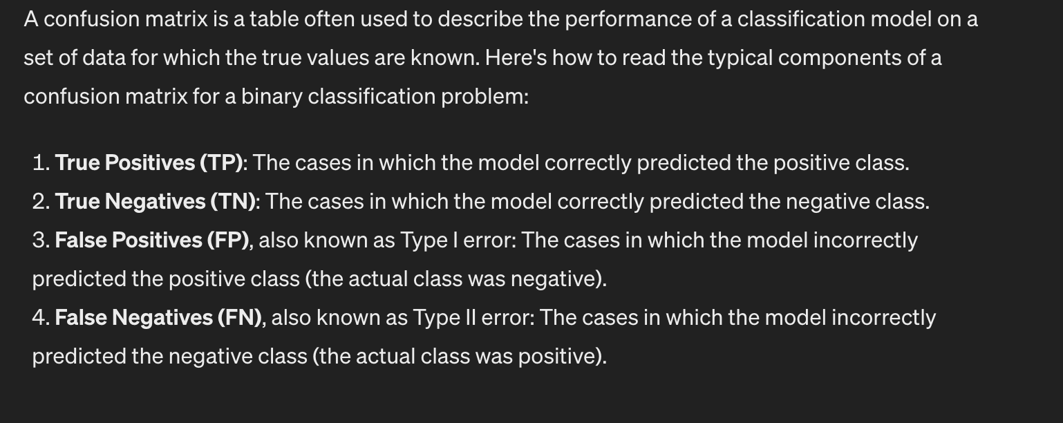
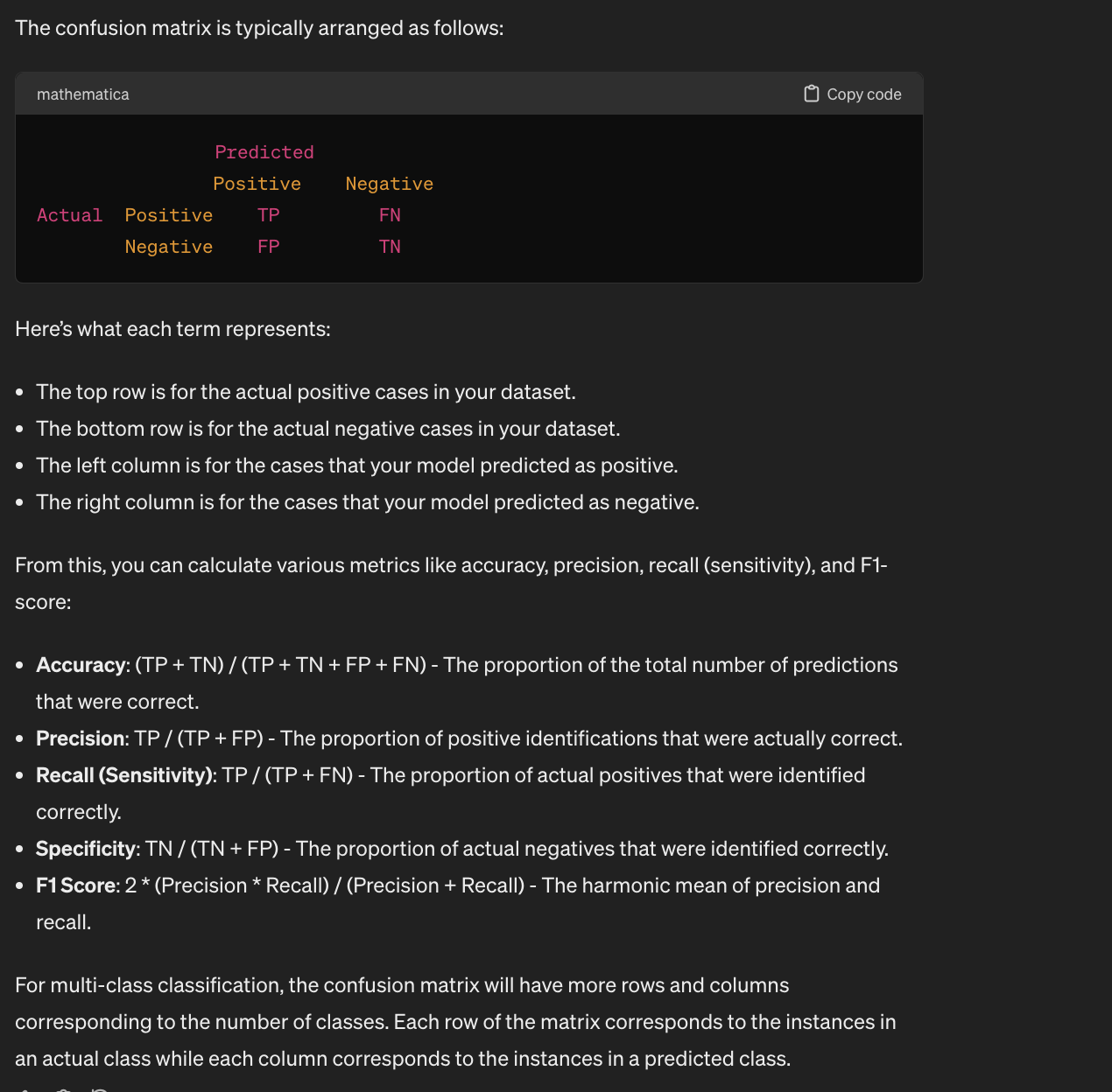
Confusion Matrix