Title: GeoQuest: Navigating QGIS’s Geospatial Tools

Description: Come learn how to enhance your GIS analysis by learning about vector geoprocessing tools in QGIS. This workshop will walk you through a variety of geoprocessing tools using different types of shapes files.

Pre Workshop:

Before the workshop please download the QGIS program to your computer using the following instructions:

1. Go to the Download QGIS website by either clicking on the linked hypertext or type in the web address below.

Website (https://qgis.org/en/site/forusers/download.html)

2. Locate your operating system in the list of download options
3. Please download the latest long term release. The long term release version of the program and the most stable at this time. By using this version of the program we will all see the same type of interface and there should be less confusion as we work through this workshop.

Workshop:

Goals:

1. Become familiar with different types of commonly used geoprocessing tools.
2. How to convert a coordinate reference system and why projection is important for geoprocessing.

Getting the Data

In preparation for this tutorial data was gathered from a few different sources. The majority of data cleaning and standardization has been completed. If there are questions about the data gathering, standardization, and cleaning please let the instructor know.

Downloading Data

First things first, we need to have data to work with. I have provided a link to all the data sources we will be using below for anyone who wants to look at the data portals and the descriptions. However, to save some time please use this link: https://drive.google.com/drive/folders/1wV8ExmUEZ0fRpoWqyTgfx-Y-lBojXTZn?usp=sharing  to get all the data. This Google folder I have created to hold what we need. To download the files from the Google Folder:

1. Go to the folder
2. In the upper right hand corner is a Download All button click there.
3. This will now download a zip file to your computer.

Unzipping a file

1. Find the downloaded folders on your computer (most likely in your downloads folder)
2. Right click on the folder and select “Extract All”
3. Save the folder in a location you will remember where it is and by a name you can remember.

1. I suggest creating a new folder every time you start a new GIS project where you can save data associated with the project.

Data from this workshop came from:

• Florida Geographic Data Library
• Florida Geospatial Open Data Portal
• Tallahassee - Leon County GIS
• Open Topography

Spatial Analysis and Geoprocessing Tools

Part 1: Buffers

Buffers are a zone that is drawn around any point, line, or polygon that encompasses all of the area within a specified distance of the feature. Meaning it can be used to help illustrate rivers flood zones, visually identifying objects within a certain distance of other objects and so on.

1. Load the files:

1. Waterways_Florida
2. Florida

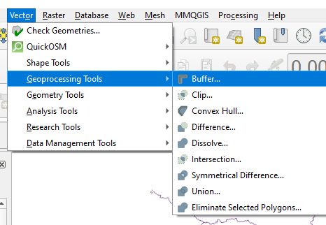
2. In the menu bar select Vector > Geoprocessing Tools> Buffer

3. In the window that opens up make sure the Waterways_Florida is selected in the Input layer. Before we move on, notice the warning symbol that appears on the Distance line. This warning symbol informs us that this layer is drawn in the WGS 84 (WGS = World Geodetic System and is considered a standard for GPS) which is a Geographic Coordinate System. Geographic Coordinate Systems places the data on a round surface so the units end up being in degrees. This means that the distance is harder to calculate because each unit of measure would need to be converted to degree.To work around this problem we will convert the coordinate reference system (CRS) to a Projected Coordinate System which will let us draw buffers in more conventional units of measure.  

1. Geographic Coordinate System defines where on the earth the data is located and drawn. Projected Coordinate System tells the program how to draw the data on a flat surface (Smith 2020).
2. For additional details read the ArcGIS Blog post Geograpvs. Projected Coordinate Systems at https://www.esri.com/arcgis-blog/products/arcgis-pro/mapping/gcs_vs_pcs/ .

4. Lets check the layers current CRS. Right click on the layer > Layer CRS > Set Layer CRS

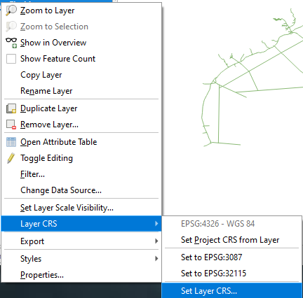
5. In the pop-up window use the filter bar to search for 3087. A list of different projection systems will appear and if you look at the descriptions of the projection system you will see there are different units of length. For today we are going to choose NAD83(HARN)/Florida GDL Albers EPSG:3087. Click this projection system and then click okay.

1. You may need to expand “Projected” then expand “Alders Equal Area” see example below

6. A pop-up window will appear. This window is saying that there multiple ways this data can be converted from to the new CRS. We can accept the default for today so just click okay.
7. When you get back to the map canvas you will see that the layer has disappeared. This is due to the redrawing, simply right click the layer and select Zoom to Layer.
8. Now go back to the Buffer tool (step 2). You should see the warning symbol is gone and the distance unit is now set to meters.

9. For some reason (it may be a glitch in the program I am not sure why) the buffer is still being drawn in degrees. The work around I have found looking on various forums such as the QGIS Reddit, StackOverFlow, and others we need to export the layer as a new layer with a the correct CRS (The fix we are using was found on this forum thread https://www.reddit.com/r/QGIS/comments/e49d2w/my_1meter_buffer_is_too_big_how_can_i_fix_this/).

1. Right click on the original waterways layer and Export> Save Feature As. New window opens up,

1. Use the drop down menu for format and change it to “ESRI Shapefile”
2. Set the CRS to NAD83 Florida GDL EPSG 3087.
3. Give the file a new name such as Waterways-FloridaGDLAlders; I suggest making sure the file is saved to the same data folder where you keep the other data for the project.

10. With the new layer successfully exported lets set the project to the same CRS as the layer. You do this either by going the project properties or you can right click the EPSG in the bottom right hand corner of the screen. Set project CRS to NAD83 Florida GDL EPSG 3087.

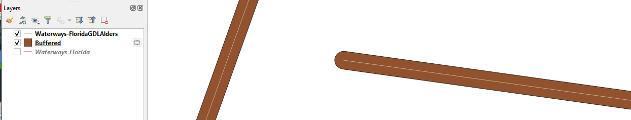
11. Now buffer the new Waterways-FloridaGDLAlders layer to 10 meters and arrange the layers so that the line layer is on top of the generated buffer layer so you can see the generated buffer zone around the line, you will need to zoom in to see the buffer.

One Side buffer

There may be occasions where you want to buffer just one side of the line, for example when planning where sidewalks would go alongside a road.

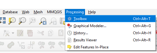
1. Go to Processing > Toolbox

2. A panel will open up on the right hand side of the screen, in the search bar search for “buffer”. Pick the “Single sides buffer” under the Vector geometry

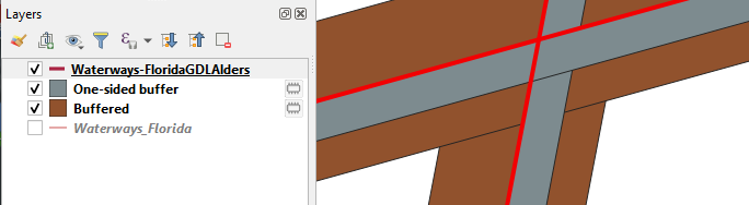
3. In the pop-up window put the Waterways-FloridaGDLAlders into the input layer, set the Buffer distance to 5 meters, and pick left or right for the buffer side. Click Run at the bottom of the window.

4. Your two new buffers should look something like this. (Note the original line was changed to red and made thicker for this image to make it easier to see the original line location).

Temporary layers

We are going to take a moment to talk about the two new layers we have created. These layers are temporary layers which means that if you do not save your work as you go when you exit the program you can lose those layers and you will not be able to add the generated layers to other projects. Additionally the names are auto generated giving very generic names. If you are creating multiple layers with these tools you should give them unique names and if you think you want to use them for other work make them permeate layers.

Rename Layer

1. Right click on the buffer layer that we created for one side of the waterways. Click on Properties
2. Under Source (on the left hand side of the pop-up window) you can change the Layer name. Give this layer the name WaterwaysGDL-5mBuffer-right.
3. Click Apply and OK

4. Go ahead and give the other layers new names.

*You can also use the rename when you right click on the layer

Saving Temporary Layers

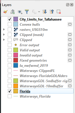
1. Right click on one of the temporary files. They are indicated with this icon in the layers panel .
2. Choose “Make Permanent”
3. In the pop-up window leave the Format set to ESRI Shapefile. Click on the three dots button and navigate to the folder where you have saved your data for this project. Give the file a name (it can be the same as the layer name if it is unique and tells you what the file is).
4. Click Save
5. Click OK
6. Now if you go to that folder on your computer you should see a new shapefile and accompanying files have been added to the folder.

Part 2: Clipping

Clipping layers is useful to reduce a dataset but cutting pieces of it out using details from another dataset, much like how you use a cookie cutter to cut pieces out of a larger sheet of dough.

Clip Vector

1. Load the files:

1. City_Limits_for_Tallahassee shape file
2. Lu_nwfwmd_2019 shape file (This is land use data from the Northwest Florida Water Management District)

2. Zoom to the Tallahassee city limits layer and make sure it is on top of  the lu_nwfwmd_2019 polygons. (Reorder the layers in the layers area).
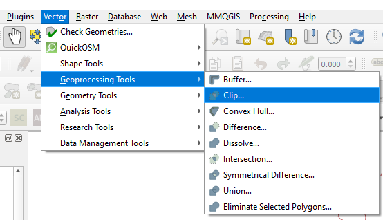
3. Lets clip the land use layer to the shape of Tallahassee. Vector > Geoprocessing Tools > Clip

4. Set the Input Layer to lu_nwfwmd_2016 and the Overlay Layer to City_limits_for_Tallahassee

5. When you hit run you should get a message that says the land use layer has invalid geometry. An invaild geometry occurs when there is a problem with the object's shape definition (the geometry). We are going to use the QGIS built in algorithm to fix the invaild geometries.

Fixing invalid geometry

1. Open the Processing Toolbox (we did this when we wanted to do a one sided buffer). In the tool box search for “Check validity”

2. Put the land use layer in as the input layer and set method to the GEOS. When the check is done running three new layers will be generated: Valid output, Invailid output, and error output.

3. The Error output layer will give us the details of which areas have the problem. Open the attribute table for this layer. Lucky for use the problem points are the same type of error, a “Ring self- intersection” error. In the Processing Toolbox search for “fix geometries”

4. In the dialog box put the lu_nwfwmd_2019 as the input layer and click Run.

5. When the program is done running a new layer will be generated called “Fix Geometries”. Turn off the three layers made in the check validity step.

Finish clipping vector

1. Open the vector Clipping tool. Set the input layer to Fixed geometries and the Overlay layer to the Tallahassee city limits.

2.  A layer called Clipped should have been added to the project. Turn off the Fixed Geometries and the lu_nmfwmd_2019 layer. Turn the Clipped layer on and off to see how it does fit in the Tallahassee city limits.

3. Not only was the visual clipped but the attribute table was reduced as well. Open the attribute tables for both the clipped layer and the lu_nwfnmd_2019 layer and compare the number of features held in each table. How many features were clipped from the original layer.

Clip Raster

1. Load the files:

1.  Tallahassee Area Raster USGS10m

1. This raster was obtained from Open Topography

2. Zoom to the Tallahassee Area Raster USGS 10m layer and have Tallahassee’s city limits drawn on top of the raster layer.
3. Go to Raster > Extraction > Clip Raster by Mask Layer

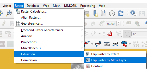
4. Since we only have one raster layer that should automatically fill in for the Input Layer. Make the Mask Layer the City Limits layer and leave everything else as is. Click Run

5. Turn off the Tallahassee Area Raster and the Tallahassee city limits to see the clipped raster.

Part 3: Convex Hull

Convex hull uses an algorithm known as the “Minimum bounding geometry” to calculate the size and shape of a bounding area that would cover a whole layer or grouped subset of features (25.1.17).

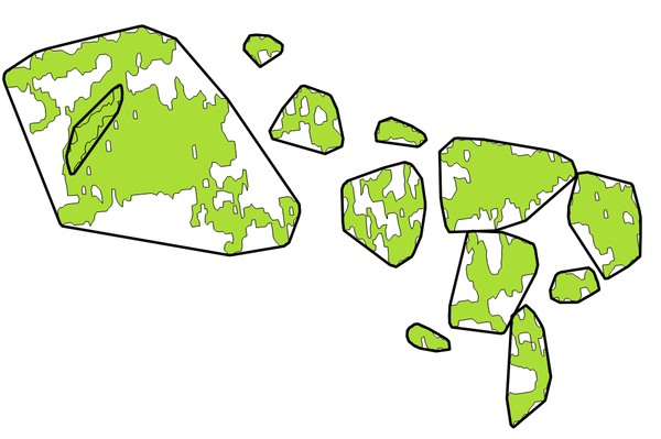
Black lines identify the convex hull for each layer feature (25.1.17)

1. Have the Tallahassee city limits polygon position as the top layer and zoom the map to that layer.
2. Go to Vector > Geoprocessing Tools  > Convex Hull

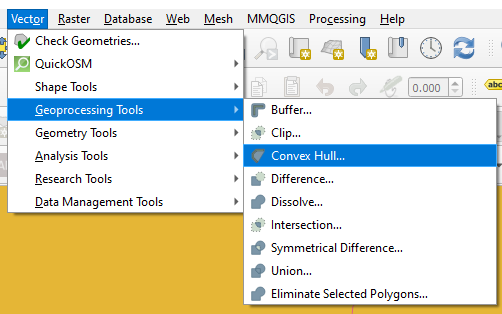
3.  In the input layer set it to the Tallahassee city limits layer. Click Run.
4. A new general shape will be drawn on top of the city limits layer. Arrange the layers so the convex hull is under the city limits. This will allow you to see how close the generated polygon tries to generalize the original shape.

Part 4: Difference

This tool allows us to determine areas that fall within one area but not another.

1. Zoom to the Florida Layer (so you see the whole state). Have the Tallahassee city limits polygon position as the top layer and turn off all other layers then the city limits and the state of Florida.

2. Go to Vector > Geoprocessing Tools  > Difference…

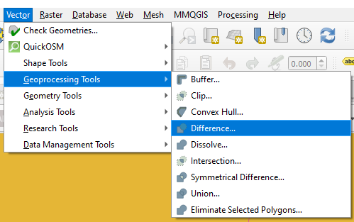
3. Set the input layer to the Florida layer and the overlay layer to the Tallahassee city limits. Click Run.
4. A new layer was generated called Difference. Turn off the city limits and the Florida layer and you can see a whole where Tallahassee would be.

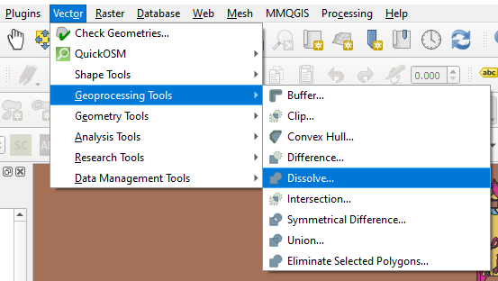
Part 5: Dissolve

Takes a vector layer and combines features into one new feature based on attributes of the same class.

1. Zoom to the Clipped vector layer we created in part 2. Open the properties window and go the symbology tab.
2. Change symbol type from “Single Symbol” to “Categorized”. Set the Value to “Level 1”. Then click Classify.

3. We have not color coded the different type of land uses in the city of Tallahassee, each polygon within the layer remains as its own feature. If we want to have a layer that groups all the polygons with the same land use type and make it as if it is one polygon even when not next to each other we use Dissolve. Go to Vector > Geoprocessing Tools > Dissolve…

4. In the dialog window make sure that the clipped layer is set as the Input layer. Then where it says “Dissolve field(s) [optional]” click on the three dots button.

5. Choose Level 1 from the list of attributes and click Run.
6. A new layer has been added called Dissolved. Open the attribute table for this layer.Now instead of all the features we had in the clipped layer we have 8 features. Click on a row so it is highlighted to see the areas where this is the same feature.

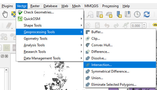
Part 6: Intersection

This is used to determine where layers overlap with one another.

1. Add the layer Building Footprints
2. Turn off all layers but the building footprints and the city limits of Tallahassee and make sure that the building footprints layer is above the city limits layer in the drawing order.
3. Go to Vector > Geoprocessing > Intersection…

4. In the dialogue window set the input layer to Building Footprints and set the overlay layer to City Limits of Tallassee. Click Run.
5. A new layer has been generated called Intersection. You may have to move it to the top of the drawing order, and look at how the layer now shows only the buildings that are within city limits.

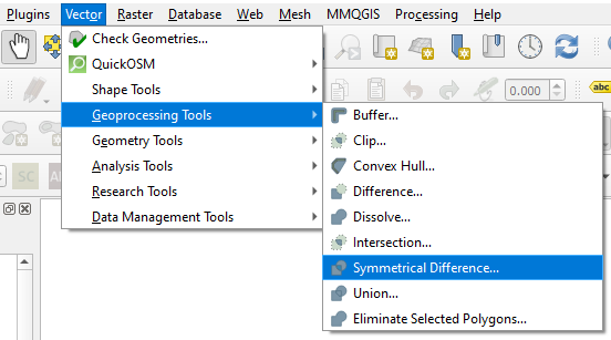
Part 7: Symmetrical Difference

This is used to create a layer where only the features from one layer are drawn because they lay outside of another layer.

1. Ensure that only the layers Building Footprints and Tallahassee are turned on and that the zoom level is set to the Building Footprints layer.
2. Go to Vector > Geoprocessing Tools > Symmetrical Differences …

3. In the dialogue window set the input layer to Building Footprints and set the overlay layer to the City limits of Tallahassee. Click Run
4. A new layer was added called Symmetrical difference. It looks like nothing changed but if we turn off the Building Footprints layer and the City Limits layer and then zoom in you will see that where the buildings that intersected with the city limits are no longer drawn. This can also be confirmed by checking the number of features in the new layer and the building footprints layer.  

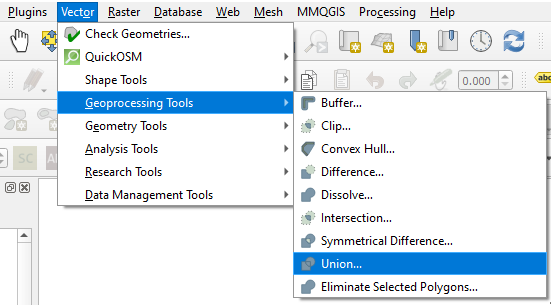
Part 8: Union

Union lets you merge two layers without removing the boundary line that separated them.

1. Load the files:

1. County Commission Districts
2. Election Precincts - Leon County

2. Zoom to one of those layers
3. Open the attribute table for the Election Precincts and take note of the attribute columns, do the same for the County Commission Districts
4. Go to Vector > Geoprocessing Tools > Union…

5. In the dialogue window set the input layer to Election Precincts and set Overlay layer to the County Commission and click Run.
6. A new layer called Union will be created. Open the attribute table what type of information has been added to the various Precincts?

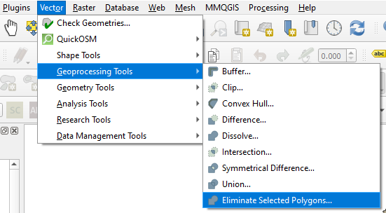
Part 9: Eliminate Selected Polygons

This tool allows for polygons in a layer to be merged together by erasing a common boundary line.

1. Set the Election Precincts to be the visible layer.
2. Use the select feature tool  to pick a few random precincts.

1. Hold the control key down to pick multiple polygons

3. Go to Vector > Geoprocessing Tools > Eliminate Selected Polygons…

4. In the dialogue box set the input layer to the Election Precincts. For the “Merge selection with the neighboring polygon with the” use the drop down menu to select “Largest Common Boundary” and click run.
5. Did the polygons you selected should now have merged with the polygon who shares the largest border with.

Reference and helpful resources

25.1.17. Vector geometry—QGIS Documentation documentation. (n.d.). Retrieved April 13, 2022, from https://docs.qgis.org/3.22/en/docs/user_manual/processing_algs/qgis/vectorgeometry.html#convex-hull 

Basic Editing Geoprocessing Tools in QGIS. (2016, January 29). https://grindgis.com/software/qgis/basic-editing-tools-in-qgis 

Florida Geospatial Open Data Portal. (n.d.). Retrieved April 19, 2022, from https://geodata.floridagio.gov/ 

Handling Invalid Geometries (QGIS3)—QGIS Tutorials and Tips. (n.d.). Retrieved April 19, 2022, from https://www.qgistutorials.com/en/docs/3/handling_invalid_geometries.html 

Looking to do a one-side buffer with QGIS v2.18.9. (n.d.). Geographic Information Systems Stack Exchange. Retrieved March 22, 2022, from https://gis.stackexchange.com/questions/243926/looking-to-do-a-one-side-buffer-with-qgis-v2-18-9 

Marsofearth. (2019, December 1). Using QGIS open up t… [Reddit Comment]. R/QGIS. www.reddit.com/r/QGIS/comments/e49d2w/my_1meter_buffer_is_too_big_how_can_i_fix_this/f98n2ag/ 

OpenTopography—Find Topography Data. (n.d.). Retrieved March 7, 2022, from https://portal.opentopography.org/datasets 

Smith, H. (2020, February 27). Geographic vs Projected Coordinate Systems. ArcGIS Blog. https://www.esri.com/arcgis-blog/products/arcgis-pro/mapping/gcs_vs_pcs/ 

United States Geological Survey (2021). United States Geological Survey 3D Elevation Program 1/3 arc-second Digital Elevation Model. Distributed by OpenTopography. https://doi.org/10.5069/G98K778D. Accessed: 2022-03-07