Terrestrial Laser Scanning International Interest Group (TLSIIG): Brisbane Instrument Intercomparison
29th July - 2nd August, 2013
2.1. LTER Plots at Karawatha Forest Park
2.2. Landers Hut 3 Plot at D’Aguilar National Park
6. Accommodation and Transport
1. Purpose
Coincident scans from current research and commercial TLS instruments across a range of contrasting canopy structures and scanning configurations will provide a benchmark dataset for comparison of different lidar technologies and algorithms through the TLSIIG. Advancing our understanding of differences and limitations of TLS instruments for vegetation characterisation is an important step towards developing operational methods for rapid vegetation structure and biomass assessment over large areas. Key research areas that we aim to contribute to through this TLSIIG collaboration include:
- Assess the sensitivity of canopy structure and biomass retrieval algorithms to changes in sensor properties and scan settings.
- Cross-calibration of TLS instruments to enhance post-hoc synthesis of TLS datasets and derived biophysical parameters.
- Intercomparison of biophysical parameter retrieval (e.g. LAI, water content) derived from single and dual-wavelength lidar processing.
- Investigate the implication of instrument specifications on the separation of woody and non-woody canopy components.
- Provide a dataset that can be readily used to parameterise 3D forest reconstruction for radiative transfer simulations (e.g. MCRT).
2. Study Site Background
2.1. Brisbane Conditions
The climate in Brisbane is not overly offensive. Typical conditions for July/August (typically the driest time of year) are:
- Maximum temperature 20.6 - 21.7 °C, 69.08 - 71.06 °F
- Minimum temperature 9.5 - 10.0 °C, 49.1 - 50 °F
- Maximum wind gust speed 85 - 105 km/h
- Mean rainfall 43 - 63 mm
- Median rainfall 34 - 40 mm
- Average 7 days of rain each month
As it is winter in Australia in July/August, we can expect only 10 hours and 50 minutes of daylight (Sunrise is ~6:30 am, sunset is ~5:20 pm, solar maximum ~11:55 am).
The best source of information on weather conditions are the Bureau of Meteorology weather and radar websites.
2.2. LTER Plots at Karawatha Forest Park
Karawatha Forest is on the southern peri-urban edge of Brisbane, covers an area of 900 ha, is 80-100 m above sea level, and is managed by the Brisbane City Council. It contains a variety of habitats from freshwater lagoons and sandstone ridges, to dry eucalypt forests and wet heath.
Between January and September of 2007 a Program for Planned Biodiversity and Ecosystem Research (PPBio) grid was established as a long-term ecological research site (LTER) in the Eucalypt forest at Karawatha Forest Park. The site is now also a Terrestrial Ecosystem Research Network (TERN) peri-urban supersite, and is maintained by Griffith University (Contact: Associate Professor Jean-Marc Hero; M.Hero@griffith.edu.au). A research grid was arbitrarily placed to cover the reserve and includes approximately 33 km of fixed transects and 33 fixed 1 ha plots at 500 m intervals. Each plot follows the elevational contour and is 250 m long by 40 m wide. Individual woody plants were tagged, identified to species level and measured for DBH, during January and February 2009.
The proposal is for the TLSIIG to visit three 1 ha plots during the course of two days. Two of these plots were also measured by TERN Auscover in February 2013 and were selected to be easily accessible and encompass different structural types.The range of stand basal area is 17 - 22.7 m2 ha-1, and crown cover projection range of 79 - 92%.
Do
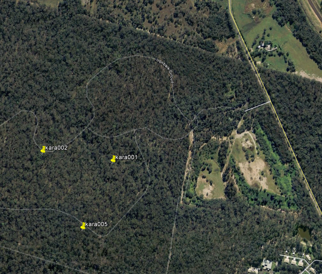
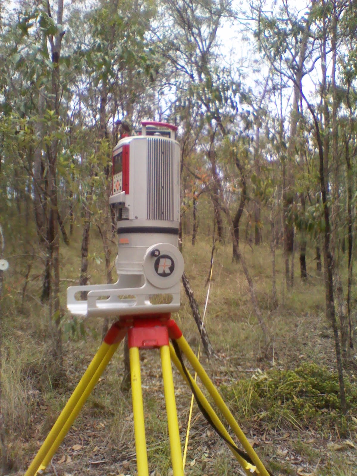
Figure 1: Left: Location of the three 1 ha TERN Auscover and PPBio plots selected for scanning in Karawatha Forest Park south of Brisbane. Right: kara001 plot centre and the RIEGL VZ400.
2.3. Landers Hut 3 Plot at D’Aguilar National Park
D’Aguilar National Park covers an area of 36,000 ha to the north-west of Brisbane city centre. The park is dominated by Eucalyptus woodland with pockets of subtropical rainforest. The Landers Hut 3 site was established by the Queensland Government Department of Science, Information Technology, Innovation and the Arts (SITIA) and is located at latitude 27.429S and longitude 152.827E (SITIA plot code: gold0101). The site is a Eucalyptus forest stand with high grass cover, fine litter and woody debris present. Although some large stems have been removed in past logging, the site includes many mature trees with heights ranging up to 35m.
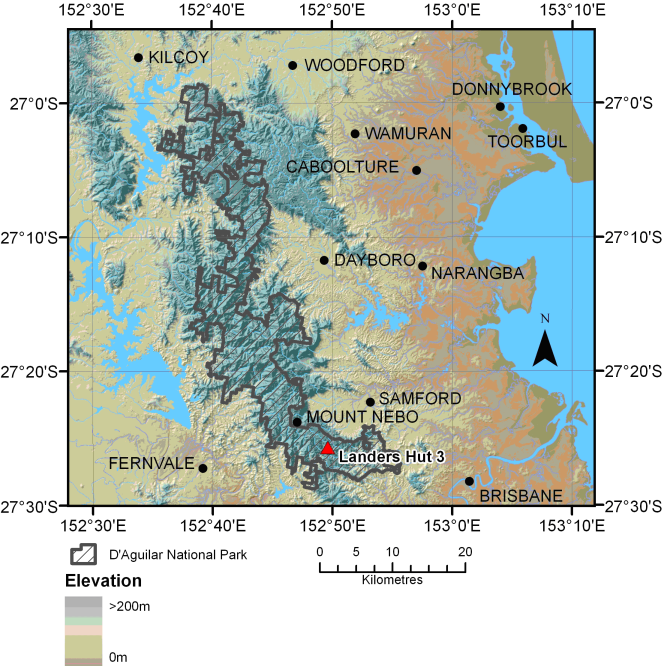
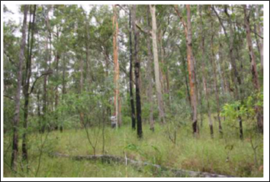
Figure 2: Left: Location of the TLS trial site (Landers Hut 3, SITIA code: gold0101) in D’Aguilar National Park to the north-west of Brisbane. Right: Site photograph.
3. Instruments
The scanners participating in the TLSIIG collaborative campaign are listed in Table 1. An additional method currently in use to measure 3D vegetation structure, Ausplots Photopoint, will also participate. It is hoped that data from all activities during the campaign (field measurements and laser scanning) will be made freely available through the TLSIIG website.
Table 1: Participating TLS and their specifications.
Instrument | SALCA[3] | RIEGL VZ400[4] | UMB CBL (RIT SICK) | FARO FOCUS 3D | |
Institution | Boston University | University of Salford, UK | DSITIA | University of Massachusetts, Boston | University of Southern Queensland |
Contact | Alan Strahler Crystal Schaaf | Mark Danson Rachel Gaulton Steve Hancock | John Armston Kasper Johansen | Crystal Schaaf | Zhenyu Zhang |
Ranging Technique | Time-of-flight | Time-of-flight | Time-of-flight | Time-of-flight | Phase-shift |
Recorded Data | Waveform | Waveform | Multiple discrete return Waveform[5] | 1st and 2nd discrete return | Single discrete return |
Scan Configuration | 0-119 zenith | 1.6-97.6 zenith 0-360 azimuth | 30-130 zenith[6] 0-360 azimuth | 0-135 zenith 0-360 azimuth | 0-160 zenith 0-360 azimuth |
Wavelengths | 1063.85 nm 1547.76 nm | 1063.4 nm 1545.4 nm | 1550 nm | 905 nm | 905 nm |
Angular Resolution | 1 mrad 2 mrad 4 mrad | 1.05 mrad zenith 1.05, 2.1, 4.2 mrad azimuth | 0.04-5.03 mrad zenith 0.04-8.73 mrad azimuth | 0.25 deg 0.50 deg | ≥0.157 mrad |
Waveform Sampling Interval | 7.5 cm | 15 cm | 30 cm | N/A | N/A |
Beam Divergence | 1.25 mrad 2.5 mrad 5 mrad | 0.56 mrad | 0.35 mrad | 15 mrad | 0.16 mrad |
Beam Exit Diameter[7] | 6 mm | 2.4 mm 3.6 mm | 7 mm | 8 mm | 3.8 mm |
Detector FOV | 5 mrad | 2.67 mrad | Not available | Not available | Not available |
Pulse Length (FWHM) | 5.1 ns 5.12 ns | 1 ns 3 ns | 3 ns | Not available | N/A (CW) |
Pulse Energy | 0.6 μJ 0.6 μJ | 0.5 μJ (1664 nm) 5 μJ (1550 nm) | 0.48 μJ | Not available | Not available |
Laser Class | 3R | 3R | 1 | 1 | 3R |
Pulse Rate | 20 kHz | 5 kHz | 100 kHz 300 kHz | 50 Hz 25 Hz | Not available |
Effective Measurement Rate | 2,000 p/sec | Not available | 42,000 p/sec 122,000 p/sec | Not available | 976,000 p/sec |
Weight | 22 kg | 15 kg | 9.6 kg | 1.1 kg | 5 kg |
Min. Range | ~0 | ~0 | 0.5-1.5 m | Not available | 0.6 m |
Max. Range | 100 m (10% ρ) | 150 m (10% ρ) 105 (10% ρ) | 200 m (10% ρ) 120 m (10% ρ) | 18 m (10% ρ) | 20 m (10% ρ) |
4. Experimental Plan
4.1. Sampling Design
Four Eucalypt woodland plots on sloped terrain at two sites have been selected for the scanner comparison experiment. Karawatha Forest Park and D’Aguilar National Park have distinct vegetation structure which may help to highlight differences in the performance of each instrument.
The sampling design is shown in Figure 3. Instrument positions may be shifted by a few meters to avoid near range stems or shrub foliage (minimum distance is 1.5 m for the Riegl). The height of the optical center for each instrument height should be as consistent as possible. Scan locations will be staked and each scanner should be positioned directly above these points.
For registration of scans to each other and to airborne data, up to 20 reflector targets (10 cm cylinders) will be placed at locations that minimise occlusion. Additional reflector targets (5 cm disks) will be placed in the Riegl tilt scan overlap if necessary. Based on known plot centre coordinates, the derived coordinates for targets from the Riegl will be used in place of surveying the targets in the field. Targets will be set up in the morning at each site and not touched for the rest of the day.
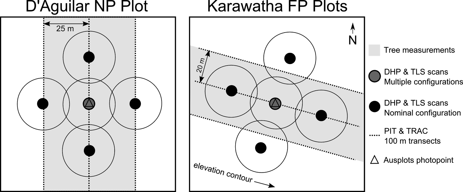
Figure 3: Sampling design for field plots at D’Aguilar National Park and Karawatha Forest Park showing the location of the scan positions and field measurements. At some sites only the centre position will be scanned.
4.2. Field Measurements
Existing field measurements at each study site are listed in Table 2. TERN Auscover field measurement protocols were followed for Karawatha Forest Park. The individual trees measured were previously determined from a 360 degree sweep using an optical wedge prism or an angle gauge. In addition, the height and DBH of all trees >1cm DBH have been measured within the 240 m by 40 m LTER field plots. The DBH, height, and crown dimensions of all trees within the 100 m by 50 m field plot were measured for the D’Aguilar National Park site in 2011.
Additional measurements to be measured during the exercise include LAI, leaf water content, plant radiometry, clumping index, and leaf size/shape. Participants may have an interest in collecting additional measurements during the field campaign in July and this should be discussed during planning. Care need to be taken to ensure field measurements do not interfere with the scanning.
Leaf Area Index (LAI) and clumping index
Digital Hemispherical Photography (DHP) will be used to derive independent estimates of LAI. The DHP will be acquired at each scan position and height. Time permitting, DHP will also be acquired at 10 m intervals along each of the PIT/TRAC transects. Processing of the DHP images will be completed using CanEye. Wood-to-total-plant-area ratios will be derived from field measurements or, if possible, CanEye processing.
Assuming clear sky conditions and sufficient time, TRAC measurements will be acquired for estimation of the element clumping index. These can be used in combination with DHP to improve estimates of LAI. A minimum of two 100 m transects will be acquired at a bearing orthogonal to the solar azimuth angle. 100 m tapes will be laid out with markers placed at 10 m intervals. The transects will be acquired at a time when the solar zenith angle is between 30 and 60 degrees.
Plant radiometry
At each site multiple samples of foliage and bark from several crowns of dominant species will be collected. To increase the number of samples an ASD leaf clip and contact probe will be used, however this will result in estimates of conical reflectance. These will be compared against a much smaller sample of hemispherical reflectance estimates derived using an integrating sphere. The number of samples that are practical to harvest and measure will be determined in the field.
Leaf water content and size/shape
Foliage clumps from a number of scanned trees will be harvested for estimation of leaf water content and size/shape. Wet weights of harvested leaves will be measured in the field using an electric balance and stored in plastic bags. Sampled leaves with a scale and white background will be imaged using a flat-bed scanner at ESP following fieldwork. The samples will then be placed in a drying oven for two days at 60 degrees C for subsequent measurement of dry weights.
At the D’Aguilar National Park site, a 1m3 volume of foliage will be harvested from a suitable Eucalypt tree. Leaf area and dry weights will then be derived from a stratified sample of these leaves. A relationship between the two will be derived, and all leaves will be weighted for conversion to LAI.
Table 2: Existing field measurements at each scan location. Measurements to be collected during the activity are highlighted in red.
Measurement | Karawatha Forest Park | D’Aguilar National Park |
Stem diameter | LTER (> 1 cm @ 1.3 m) Auscover (angle gauge sampling) | Yes (> 5 cm @ 0.3 and 1.3 m) |
Crown top height | Yes | Yes |
Crown base height | Yes | Yes |
Crown opacity | No | Yes (vertical Pgap) |
Crown diameter | Yes | Yes (major/minor axis) |
Stem locations | No | Yes |
Leaf area index | Yes (indirect) | Yes (indirect) |
Leaf biochemistry
| No | No |
Leaf/wood spectra Soil/litter/grass | No | No |
Floristics | Yes | Yes |
Element clumping index (TRAC/DHP) | No | Yes |
Point intercept transects
| Yes | Yes (monthly) |
Leaf size/shape | No | No |
4.3. Scanning Configurations
Calibration Scans
Prior to field scanning (Monday 29th July at ESP), DWEL and SALCA laser measurements in non-scanning mode will be acquired using reflectance panels of varying brightness at a range of distances from 5 m to 70 m. Due to the larger footprint of the SALCA and DWEL instruments, at least a 50 cm by 50 cm panel is required for laser measurements up to 100 m range. A visible marker laser will be used to ensure the point spread function is centred over the panel. Repeat measurements will be acquired to compute an estimate of the error and test stability of the pulse properties. Measurements from the Riegl VZ400, Faro Focus 3D, and CBL will be sampled by averaging all pulses that fully intercept the calibration panels (pulses will be selected using the intensity image). The standard deviation will also be computed as an estimate of the error.
An instrument intensity calibration experiment will take place on the Sunday afternoon and/or evenings, to minimize chance of disturbance and stray light. The primary calibration target will be 25 cm white spectralon panels with calibration certificates. Secondary calibration targets are being made from stiff painted boards. Matte paints are being tested for nominally 10%, 25%, 50% and 99% (mixed with barium sulphate) Lambertian reflectance (avoiding specularity is key), and spectral flatness at the relevant wavelengths, 905, 1064, and 1550 nm.
Field Plot Scans
Details of the scan configurations are listed in Table 3. The objective was to have as near equivalent scan configurations as possible for each scanner at each location. Options to further customise DWEL and SALCA scanning configurations to better meet this objective will be discussed prior to fieldwork. Waveforms from the RIEGL VZ400 will be sampled and/or aggregated in post-processing to match the scan configuration of the DWEL, SALCA and CBL instruments.
Multiple scan configurations will be tested at the centre scan position of each field plot. A nominal scan configuration will be used for four additional scan positions at two Karawatha Forest Park plots and the D’Aguilar National Park plot. The RIEGL VZ400 will also be used to scan a sample of individual trees for construction of 3D tree models.
To maximise scanning time, field plots at Karawatha Forest Park will be acquired simultaneously with DWEL and SALCA at separate plots. Due to limited time and proximity of scan locations at the D’Aguilar National Park plot, it is proposed that DWEL and SALCA scan simultaneously at opposite corners (100 m apart). North and south corners will be scanned first as coincident with stem measurements.
All Instruments will be plumbed over the scan location marker (a stake driven to ground level with nail at the centre) and set up such that the optical centre is at a height of ~1.7 m. If possible, instruments will be oriented so that the scan start azimuth is as close as possible to true north.
For each SALCA and DWEL scan, a large panel with six 30cm by 30cm sub-panels of nominally 15%, 30%, 45%, 60%, 75%, and 99% reflectivity will be placed within the FOV of the scanner, and then moved (at a constant distance from the scanner) around as the scan proceeds so the board appears about 4 - 6 times within a given hemispherical scan.
Wind and temperature measurements will be recorded using a portable weather station at the field sites during each scanning day.
Table 3: Summary of scan settings to be used for multiple scan configurations. The nominal scan configuration for scans at multiple positions is highlighted in red. The nominal scan configuration is intended to generate equivalent scan configurations for each instrument.
Setting | DWEL | SALCA[8] | RIEGL VZ400 | UMB CBL | FARO FOCUS 3D 120 |
Minimum number of scans | 3 | 2 | 2 | 2 | 3 |
Angular resolution[9] |
|
| 0.06 deg (1.05 mrad) |
| ≥0.157 mrad |
FOV | 0-119 zenith | 1.6-97.6 zenith 0-360 azimuth | 30-130 zenith[11] 0-360 azimuth | 0-135 zenith 0-360 azimuth | 0-160 zenith 0-360 azimuth |
Pulse rate | 2 kHz | 5 kHz |
| 1. 25 kHz | 976 kHz |
Beam divergence |
| 0.56 mrad | 0.35 mrad | 15 mrad | 0.16 mrad |
Quality (integration time) | N/A | N/A | N/A | N/A |
|
Scan time |
|
| 1. 5 min 2. 10 min |
|
|
Radial nominal ocular hazard distance | TBA | TBA | 0 m | 0 m | TBA |
5. Fieldwork Schedule
A full program for the week can be found here. The current fieldwork schedule may be amended if interrupted by poor weather. Wet and windy conditions will be avoided. If conditions are unfavourable for the planned scanning days then we will try to reschedule. The field equipment list (including personal protective equipment) can be found here.
The D’Aguilar National Park site cannot be accessed without a key and requires 4WD. Minibus transport from ESP to the Mt Nebo Road Winery is available. Three Queensland Government 4WD vehicles will transport participants and instruments to the field plot from there (~20 min). The departure/arrival point each day will be the EcoSciences Precinct Building at 41 Boggo Rd, Dutton Park QLD.
The Karawatha Forest Park can be accessed using normal 2WD vehicles. The meeting point will be at the Acacia picnic area, which can be accessed from Acacia Road, Karawatha (toilet facilities available). Gates open at 6am and close at 6pm.
The risk of dangerous animals is very low but senior staff with first aid training, first aid kits, and mobile phones will be present at each field plot. Snake are generally inactive in these cooler months. Using insect repellents on exposed skin, wearing light coloured clothes, long pants/shirt and gaiters, and regular checks will minimise the risk of ticks. Incidence of tick-borne diseases is very low in Australia (http://www.publish.csiro.au/?act=view_file&file_id=NB11025.pdf) – allergic reactions are probably the biggest risk. The following links provide some information on management of any cases:
6. Accommodation and Transport
Transport between the field sites and Boggo Road Ecosciences Precinct will be available each day. Scanners and other field equipment may be stored at the Ecosciences Precinct, which has 24 hour security. Participants are otherwise expected to organise their own transport and accommodation. Some basic walking distance (<30 min) accommodation options close to Ecosciences Precinct include:
- http://www.ambassadormotorinn.com.au
- http://dianaplaza.com.au
- http://www.hotelchino.com.au
- http://www.brisbanestreetstudios.com.au
- http://www.qresorts.com.au
Park Road Train Station and Boggo Road Busway are right outside the Ecosciences Precinct, so public transport is easy if you want to stay somewhere nicer in Southbank or the city. Park Road train station has direct trains to and from the international and domestic airports. See http://translink.com.au/ for information on train, ferry, and bus services in Brisbane.
[1] TERN Auscover / CSIRO (Contact: Glenn Newnham) plan to scan at the same site in late in 2013/early 2014 using a second DWEL instrument.
[2] DWEL PiiShaper converts Gaussian beam PSF to flat-top beam PSF.
[3] The two footprints are offset by 6 urad, which leads to a difference in footprint coverage of <1% of footprint area.
[4] Wageningen University (Contact: Kim Calders) also operate a RIEGL VZ400 with waveform recording. Coincident scans have already been acquired in November 2012 for comparison.
[5] The RIEGL VZ400 digitises the received waveform in 60 ns sample blocks, with digitisation initialised by the signal exceeding an unknown noise threshold. Only waveform sample blocks that deviate from the system waveform shape are recorded (deviation threshold is configurable).
[6] The 0-30 degree zenith angle range for the RIEGL VZ400 may be acquired using a tilt-mount.
[7] Beam diameter at 1/e2.
[8] The angular resolution of SALCA is constant in zenith (1.05 mrad) and variable in azimuth.
[9] The DWEL and SALCA finest angular resolution scans (~1 mrad) will only be for a 20-30 degree sector that encompass a single tree.
[10] Two 30 minute scans are required due to a filter change to account for laser power differences.
[11] A second scan using a 90 degree tilt mount will be used to sample the 0-30 deg zenith range.