Face Recognition via Convolutional Neural Network

Mengsu Chen  &  Mi Yan

Fall 2015 ECE 5554/4984 Computer Vision: Class Project

Authors in Alphabetical Order

Virginia Tech

We propose a face recognition pipeline consists of two recent proposed algorithm: a face alignment algorithm based on regressing local binary features (Ren et al. 2014) and a face representation algorithm based on deep convolutional neural network (Sun et al. 2014). Our results show that these two new algorithms have considerable potential in face recognition under unconstrained conditions.

Teaser figure

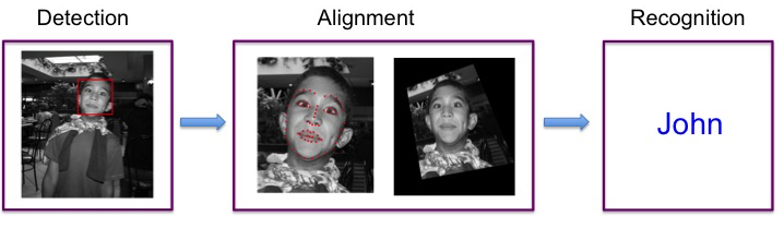
Figure 1. Pipeline of face recognition.

Introduction

Face recognition has been a standing problem for many years. The traditional solutions in the last decade are to extract hand-crafted features, such as SIFT, LBP, HoG. However, many parameters need to be carefully tuned, making this approach usually not robust to the variation of  input images. In this project, we would like to try a new approach based on convolutional neural network (CNN).

Approach

Face Detection: Viola-Jones Detector

The first step of face recognition is to detect faces in input images. This is done by using the Viola-Jones algorithm. It detects a list of bounding boxes of potential face regions, in which the initial guess facial landmarks are placed.

Face Alignment: Local Binary Feature Regression

Local binary features regression (Ren et al. 2014) is one the state-of-art algorithms for face alignment which is both highly accurate and extremely fast. This approach has two novel components: a set of local binary features, and a locality principle for learning those features. The locality principle guides us to learn a set of highly discriminative local binary features for each facial landmark independently. The obtained local binary features are used to jointly learn a linear regression for the final output. The overview of this approach is illustrated in Figure 2.  

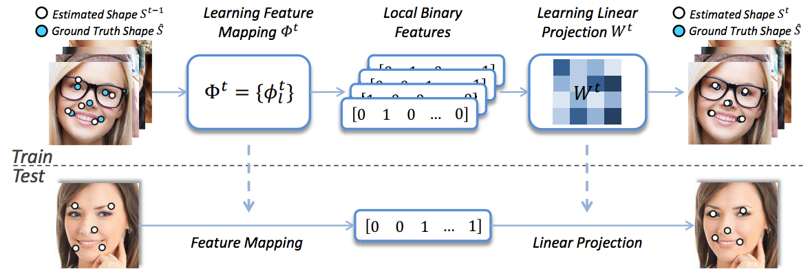
 Figure 2. Illustration of the implementation of local binary feature regression.

Face Representation: Deep Convolutional Neural Network

CNN is demonstrated to be very successful in generic object recognition. It can extract high level (more abstract) features, therefore should be more robust than hand-crafted features. In this project, the convolutional neural network we use to extract high-level features of human faces consists of four convolutional layers(Sun et al. 2014). The first three convolutional layers each followed by a max-pooling layer. The fourth convolutional layer is added to extract more global features. Then a hidden layer is fully connected to the fourth convolutional layer and the max-pooling layer of the third convolutional layer to see multi-scale features, i.e. the more global features in the fourth convolutional layer and the more local features in the third convolutional layer. This kind of bypassing connection is to reduce the information loss in the fourth convolutional layer after successive down-sampling. The hidden layer which is a 160 dimensional vector is called DeepID layer. This 160 dimensional vector is considered to be the high-level features of the image.

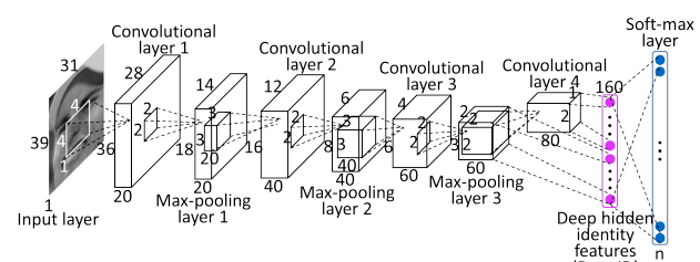
 Figure 3. Convolutional neural network used to extract high-level features

Experiments and results

Face Alignment Results and Analysis

We use a combination of the widely used  AFW, LFPW, HELEN and IBUG to train our model. All the datasets can be found here. All images in the datasets are annotated with 68 facial landmarks in Figure 4.

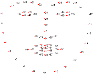
 Figure 4. A face shape annotated by 68 landmarks.

We test the trained model with the 330 test images in the Helen dataset. The error of the test images is measured as the average point-to-point Euclidean distance between the predicted shape vector and the ground truth shape. To obtain a shape invariant result, the error is  normalized by the inter-ocular distance, which is measured as the Euclidean distance between the outer corners of the eyes of the ground truth shape. The average normalized error in the test dataset is 0.0559, which is comparable to the experiment results reported in (Yang 2015).

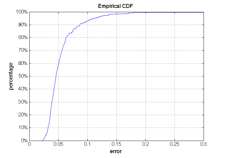
        Figure 5. Cumulative error of the test images in Helen dataset.

We plot the cumulative error of the test data set shown in Figure 5. Note that more than 90% of the test images are with error smaller than 0.1, and around 60% of the test data are with error below 0.05. So our trained model is relatively accurate to be applied in capturing facial landmarks.

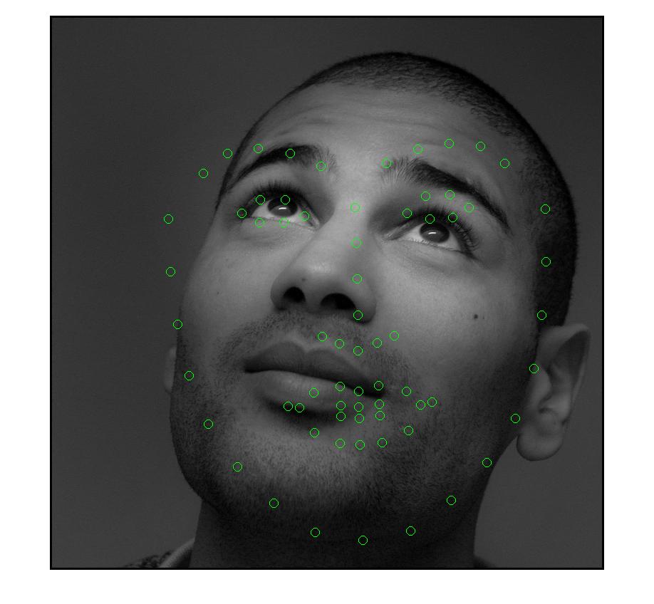
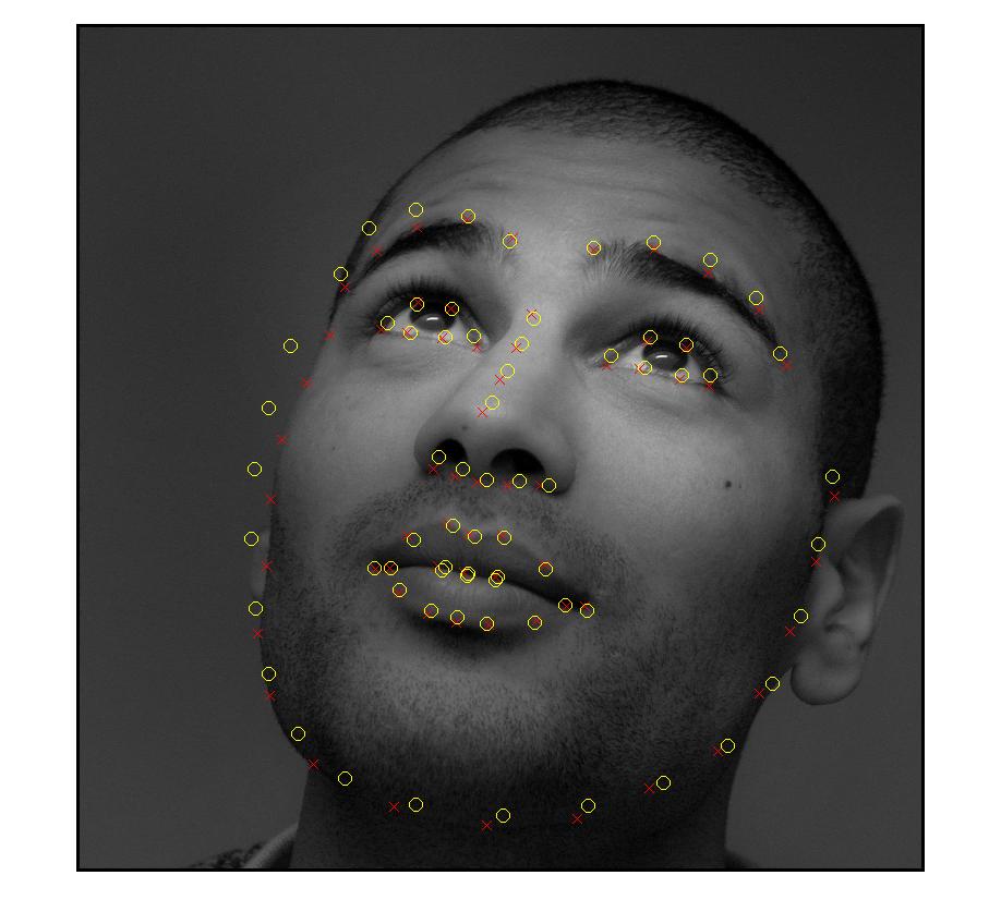
Figure 6. Comparison of initial shape (green), the predicted shape (yellow) and the ground truth shape (red).

Figure 6 shows a typical comparison between the initial guess shape, the output shape and the ground truth. It reveals that the error mainly comes from contour points with indices 1 ~ 17. Figure 7 shows the curve of a single predicted shape vector of the image in Figure 6. Note the error values for the first 17 points are larger than other points.

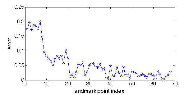
    Figure 7. Error of a single predicted shape vector in Figure 6.

After the 68 landmarks of an input image are found by our trained model, we can make them correspondences with respect to the standard landmarks in Figure 4.  We use homography transformation technique to obtain the face frontalization of the input image. A typical example is shown in Figure 8. We can use the frontalized face image for preparation of the face recognition in the next step.

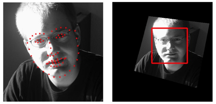
 Figure 8. Face frontalization based on landmarks.

Face Representation and Face Verification: ConvNet

We evaluate the algorithm by training the convolution neural network on YouTube Faces Dataset, which contains 3425 videos of 1595 different people, in total, has 621126 frame images. Considering the training time, we randomly pick 25 images for each person and use 20 of them as training images, 5 of them as test images. In other words, the training set has 1595*20=31900 images, the test set has 1595*5=7975 images.

The structure of the neural network is implemented based on the Theano(J. Bergstra et.al 2010) and DeepID_FaceClassify(Zhang 2015).

The training process is shown as follow with the validation error rate converges at 6%. In future, by training on larger dataset or avoiding overfitting through dropout, the error rate should be able to further reduced.

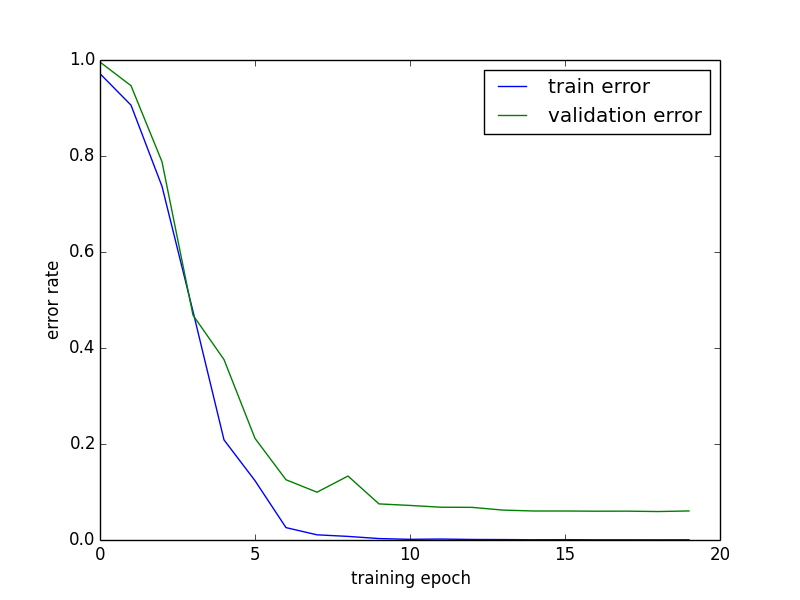
 Figure 9. Change of train and validation error rates during the training

Below are image representations of the learned 20 filters in the first convolutional layer. The gray one represents only the red channel. The colorful one represents all the three RGB channels applying to the RGB channels of the input images respectively.

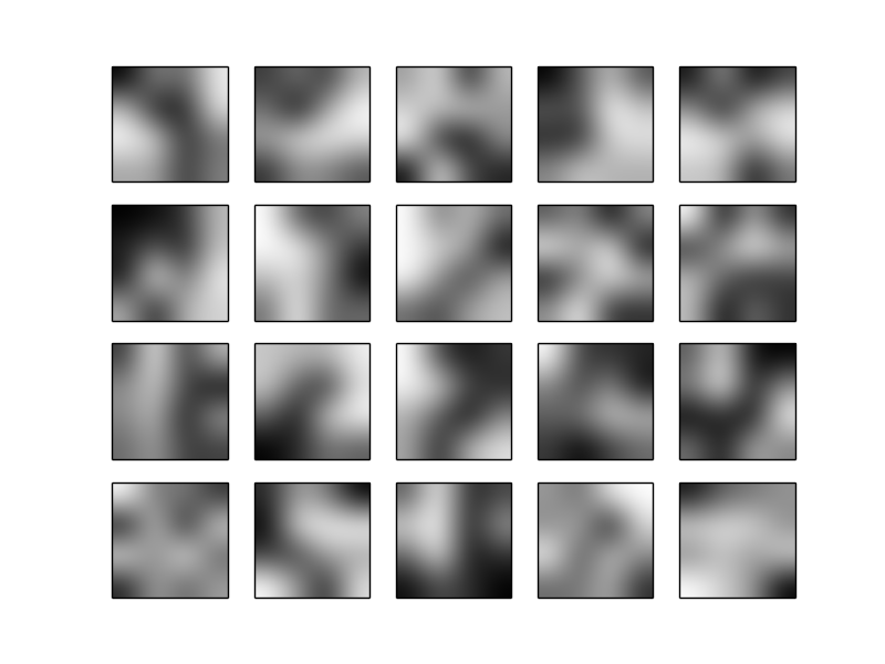
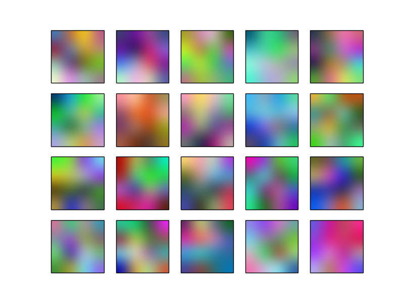
Figure 10. The 25 learned filters of the first layer (left: only red channel; right: all RGB channels)

Some examples of the learned 160-dimensional DeepID are shown as follow. Face images of the same person (vertical) have similar DeepID. Face images of different persons (horizontal) have very different DeepID. This suggest DeepID is an effective face representation.

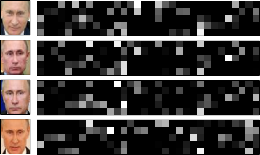
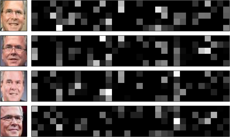
Figure 11. Examples of 160 dimensional DeepIDs

To further test the effectiveness of DeepID. We test the model, which trained on Youtube Dataset, on LFW dataset. For a quick test, we carry out face verification based on the cosine similarity of DeepIDs on LFW dataset. We pick 80 similarity thresholds uniformly distributed between 0.5 and 1 to determine the true/false positive rate on 100 pairs same/different person face images.  Keep in mind that the model is trained on Youtube Dataset where faces images are extracted from a video and very similar to each other. Also we do not retrain on LFW dataset. However, from the following graph, even the verification is based on  a naive cosine similarity, DeepID has the potential to achieve high true positive rate while keeping false positive rate low.

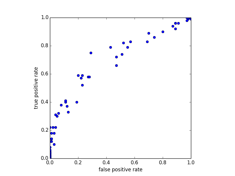
Figure 12. ROC of face verification on LFW

Reference

Jianwei Yang, Face alignment in 3000 FPS (2015), GitHub repository, In https://github.com/jwyang/face-alignment 

Ren, Shaoqing, Ren Shaoqing, Cao Xudong, Wei Yichen, and Sun Jian. 2014. “Face Alignment at 3000 FPS via Regressing Local Binary Features.” In 2014 IEEE Conference on Computer Vision and Pattern Recognition. doi:10.1109/cvpr.2014.218.

Sun, Yi, Sun Yi, Wang Xiaogang, and Tang Xiaoou. 2014. “Deep Learning Face Representation from Predicting 10,000 Classes.” In 2014 IEEE Conference on Computer Vision and Pattern Recognition. doi:10.1109/cvpr.2014.244.

Zhang Yishi. GitHub repository, In https://github.com/stdcoutzyx/DeepID_FaceClassify

J. Bergstra, O. Breuleux, F. Bastien, P. Lamblin, R. Pascanu, G. Desjardins, J. Turian, D. Warde-Farley and Y. Bengio.  “Theano: A CPU and GPU Math Expression Compiler”. Proceedings of the Python for Scientific Computing Conference (SciPy) 2010. June 30 - July 3, Austin, TX