

User Manual & Lab Activities
Table of Contents
Educational Colorimeter kit contents
Enclosure Parts (laser-cut acrylic)
Assembly of the Educational Colorimeter
Assembly of Arduino onto base plate
Optional: Assembly of Arduino with TuxCase
Upgrading from original colorimeter hardware to the new design
Programming the Arduino with the Educational Colorimeter firmware#
Educational Colorimeter software: data collection and analysis
Colorimeter concentration program
Lab 1: Introduction to Colorimetry
Lab 2: Beer's Law and Molar Extinction Coefficient
Step 1: Prepare 1 mM stock of dyes
Step 2: Preparation of standard curve
Step 3: Measure absorbance with the colorimeter and plot data
Lab 3: Ammonia and nitrate measurements
Day 0) Setting up the experiment and initial sample collection
Day 3) Prepare ammonia standard curve
Day 4) Prepare nitrate standard curve
Day 5) Measure nitrate and ammonia in samples
Introduction
Colorimeters are analytical devices commonly used in science labs to measure the concentration of a solution from its light absorbing properties. Colorimeters are extremely useful and flexible lab instruments for a wide range of science education labs. Typically, these devices are used for:
- Color and absorbance - Investigate the relationship between the color of a substance and absorption of light at different wavelengths;
- Beer’s Law - Investigate the relationship between concentration and absorbance using colored solutions (eg. food dye, copper sulfate). Calculate molar extinction coefficient;
- Nitrogen cycle - Quantify the breakdown (oxidation) of ammonia into nitrite and nitrate by nitrification bacteria;
- Water quality - Measure several water parameters such as turbidity, chlorine content, pH, water hardness, phosphate content and more;
- Population growth - Measure the turbidity of a microbial culture over time, which serves as an indicator of population growth;
- Enzyme kinetics - Measure the activity of an enzyme over time, even under different environmental conditions (temperature, pH, inhibitors, substrate);
How the Educational Colorimeter works
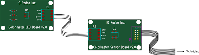
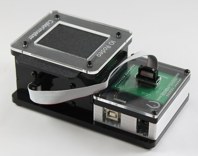
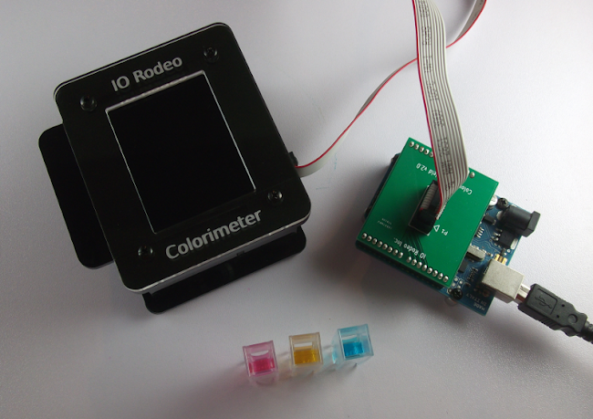
The Educational Colorimeter essentially consists of an RGB LED and a color sensor in a light-tight enclosure which is connected to an Arduino via a colorimeter shield.
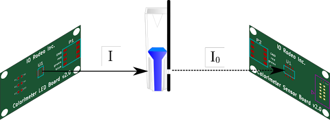
A cuvette holder in the center of the light-tight enclosure properly positions the sample between the LED and the light sensor. When the Educational Colorimeter is operating, the RGB LED illuminates one side of the sample in the cuvette using one of three different wavelengths of light: 625 nm (red), 528 nm (true green) and 470 nm (blue). On the opposite side, the light passing through the sample also passes through a slit on an inner wall of the enclosure, and falls on the light sensor. Absorbance ( ) of the sample is determined by comparing the intensity of incident light (
 ) to the intensity of light after it has passed through the sample (
 ):
):

The Educational Colorimeter uses eight (8) digital signals for normal operation. The provided Arduino shield connects 8 digital input-output (DIO) pins of the Arduino microcontroller board with the light sensor and RGB LED.

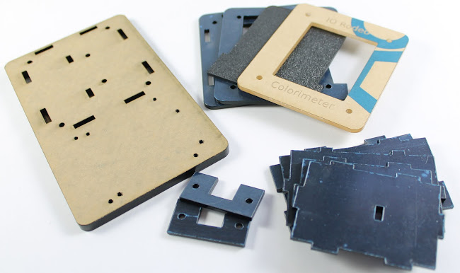
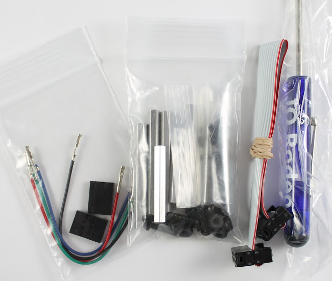
Educational Colorimeter kit contents
Each Educational Colorimeter Kit contains the electronics boards, hardware and parts listed below. The parts are described in more detail on the next 3 pages. All of the kit parts are shipped in a 1.6 L storage container. After assembly, the colorimeter fits back into the container for safe storage between uses. Note that the Arduino Uno is not listed as a kit component but is required. The Arduino Uno can be purchased pre-programmed with the kit.
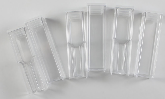
Colorimeter LED board; Colorimeter sensor board and Colorimeter shield for the Arduino. | Set of 6 cuvettes with caps (3 macro, 3 semi-macro) |
11 black laser cut acrylic parts and a clear laser cut engraved acrylic cover; | 3 bags of Hardware, ribbon cable for connecting Arduino to the colorimeter and a Philips mini screwdriver. |
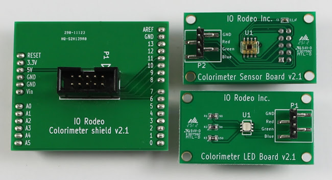
Electronics Parts
Below is a list of parts that are used to make the 3 electronics boards. Note that the electronics are already assembled with the kit. This component listing is for informational purposes only.
Qty | Description | Vendor | Part # |
1 | RGB LED PCB | --- | --- |
1 | SMT RGB LED | Digikey | 475-2822-1-ND |
1 | 4 pin SMT male header | Digikey | S1013E-04-ND |
2 | SMT resistor 90 ohm | Digikey | P90.9CCT-ND |
1 | SMT resistor 150 ohm | Digikey | P150CCT-ND |
1 | Color sensor PCB | --- | --- |
1 | SMT Color sensor | Mouser | 856-TCS3200D-TR |
1 | 4 pin SMT male header | Digikey | S1013E-04-ND |
1 | SMT 0.1uF capacitor | Digikey | 490-1577-1-ND |
1 | 5x2 shrouded header | Digikey | S9169-ND |
1 | Arduino shield PCB | --- | --- |
1 | 5x2 shrouded header | Digikey | S9169-ND |
1 | Arduino stackable header kit | Sparkfun | PRT-10007 |
Colorimeter Hardware
Bag A - Enclosure hardware
Qty | Description | Vendor | Part # |
4 | Enclosure standoffs (4-40 hex standoffs 1 ¾” long) | mcmaster-carr | 91780A038 |
2 | Cuvette standoffs (4-40 hex standoffs 1 ¼” long) | mcmaster-carr | 91780A034 |
10 | Enclosure screws (4-40 machine screws, ½” long) | mcmaster-carr | 91249A111 |
2 | Cuvette screws (4-40 machine screws, | mcmaster-carr | 91249A108 |
4 | Rubber bumpers | Digikey | SJ5012-0-ND |

Bag B - Electronics hardware
Qty | Description | Vendor | Part # |
8 | PCB screws (4-40 machine screws, | mcmaster-carr | 91249A108 |
8 | PCB Nuts | mcmaster-carr | 96537A120 |
4 | Colored pre-crimped wires (3” female-female wire) | Pololu | 1806 |
2 | Connector housing | Pololu | 1903 |
Bag C - Arduino and TuxCase hardware
Qty | Description | Vendor | Part # |
4 | TuxCase flat-head mounting screws (4-40 flat-head machine screw, 1/4" long) | mcmaster-carr | 90471A155 |
4 | Arduino mounting screws (4-40 round machine screws, 5/16” long) | mcmaster-carr | 91773A107 |
4 | Nylon standoff (Unthreaded Spacer, 1/8" long) | mcmaster-carr | 94639A610 |
4 | Nylon washer (self-retaining washer) | mcmaster-carr | 91755A205 |
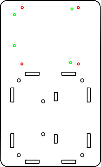
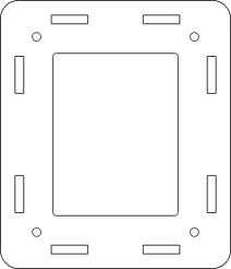
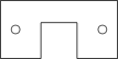
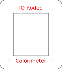
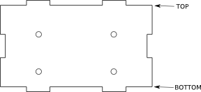
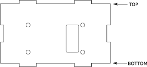
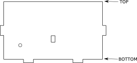
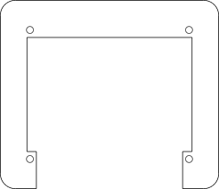
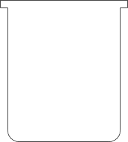
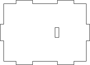
Enclosure Parts (laser-cut acrylic)
Base Plate Green holes = Arduino Red holes = TuxCase | Top Plate Cuvette Holder (2) | Clear acrylic cover |
LED Mount | Sensor Mount | Divider Wall |
Outer Slider | Inner Slider | Side Wall (2) |
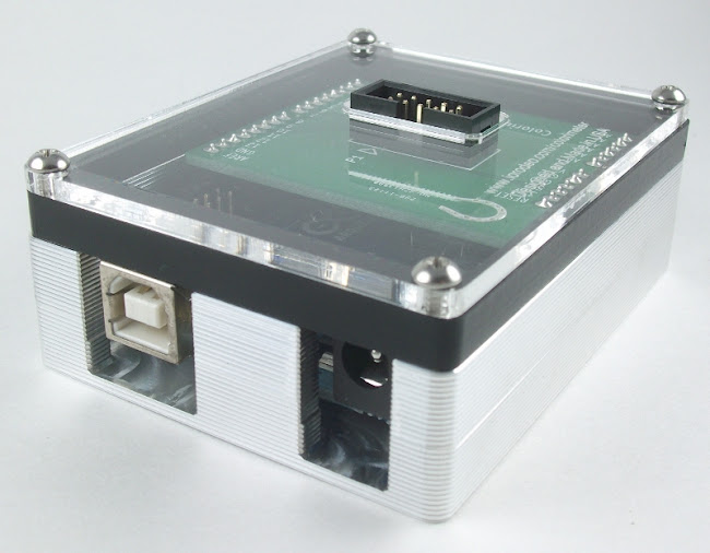
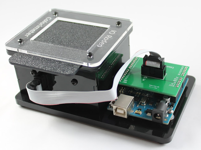
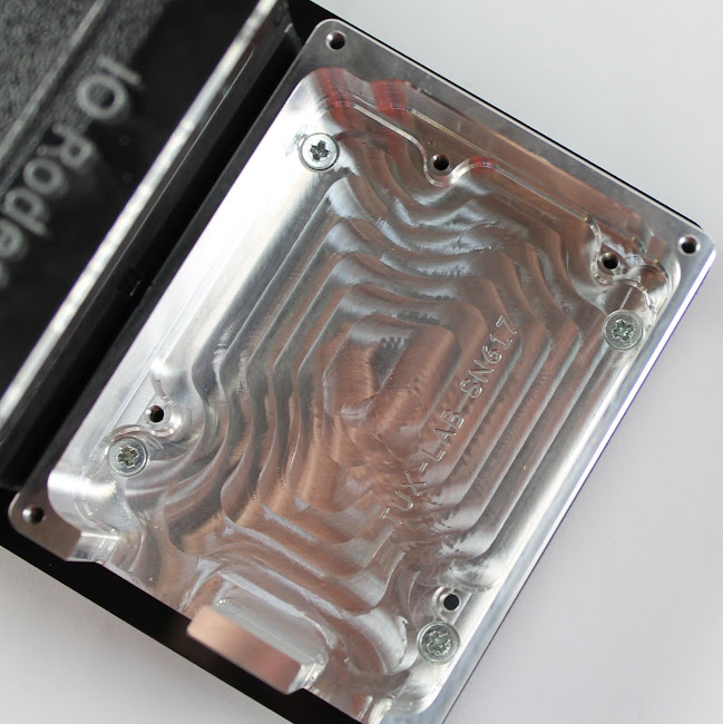
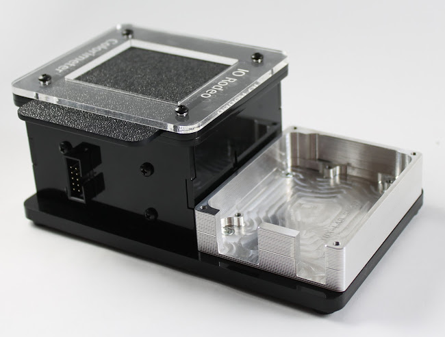
Optional TuxCase kit
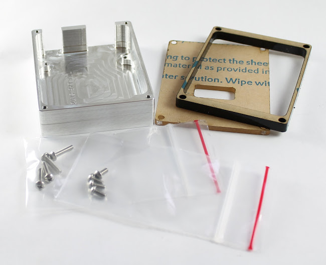
The optional colorimeter TuxCASE kit can be used as a protective enclosure for the Arduino, protecting the electronics boards from liquid spills in the lab when using the colorimeter. The aluminum enclosure is the same as the TuxCASE for Arduino. The main difference is the top - the clear acrylic top has been modified to include a cutout for the header on the colorimeter shield. A black acrylic spacer is included to raise the height of the clear top. TuxCASE is designed and manufactured by Tux-Lab. For additional information on the TuxCASE manufacturing procedure and supporting documentation, visit the Tux-Lab project page. TuxCase kit contents:
|
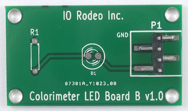
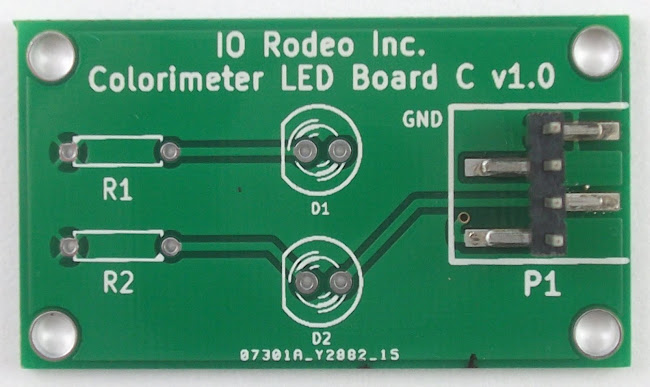
Optional: Customs LED boards
In addition to the regular RGB board that is included with the kit, there are also two additional custom boards that can be used to change the measurement wavelength. These boards can be easily swapped into the colorimeter to replace the RGB board. For example, if you only want one measurement at a wavelength other than the standard ones available, you can use LED Ver B, or for two new wavelengths, use LED Ver C.
Assembly of the Educational Colorimeter
Before starting
- Review the guides on the previous pages to easily identify the laser cut parts (highlighted in bold below);
- Peel off the protective backing from the laser cut acrylic parts. This will be either brown paper backing (clear and ¼” black) or blue plastic on most of the ⅛” black acrylic parts;
- Sort and identify the hardware parts.
Assembly of the colorimeter
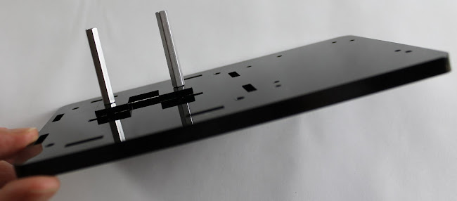
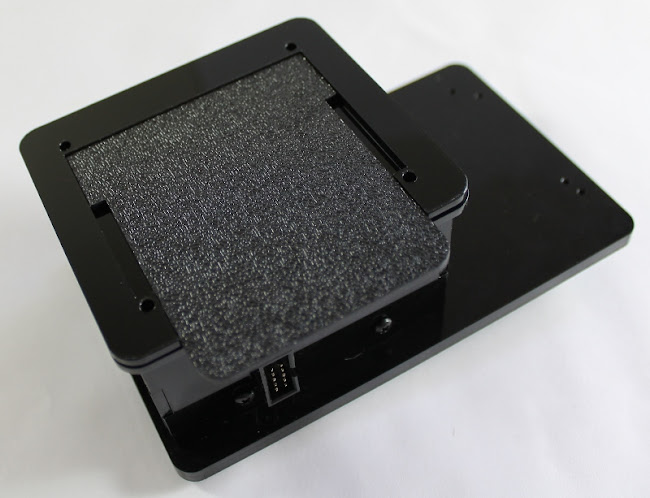
Step 1. To begin assembly of the enclosure, you will use the hardware in Bag A. After removing the paper backing from the base plate, place two of the enclosure screws through the two center holes. Secure in place with tape. Flip the base plate over and place one of the small C-shaped cuvette holders on the base plate with the cutout facing the two rectangular slots in the center of the base plate. Screw the two cuvette standoffs in place.
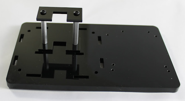
Step 2. Mount the second C-shaped cuvette holder onto the standoffs with the two shorter cuvette screws, with the same orientation as the previous cuvette holder.
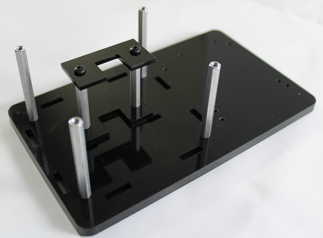
Step 3. Keeping the same orientation of the base plate, place one enclosure standoff on each corner and secure in place with an enclosure screw.
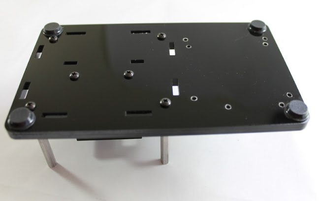
Step 4. Flip over the base plate, and place a rubber bumper on each corner.
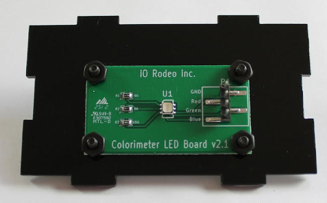
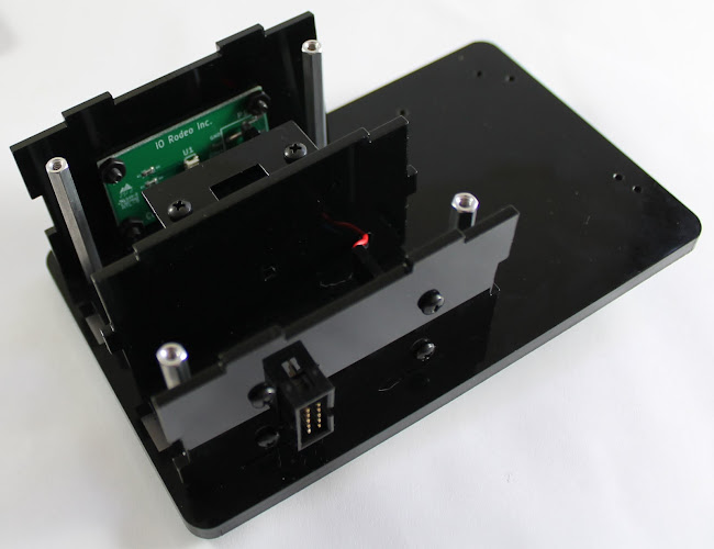
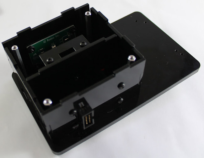
Step 5. To begin assembly of the colorimeter electronics, you will use the hardware in Bag B. Mount the Colorimeter LED Board onto the LED mount. Make sure that the placement of the board is close to the bottom edge of the LED mount as shown in the image below. Secure in place with four PCB screws and four PCB nuts.
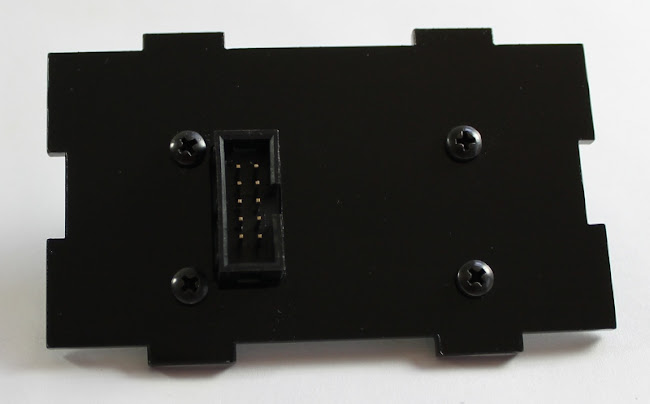
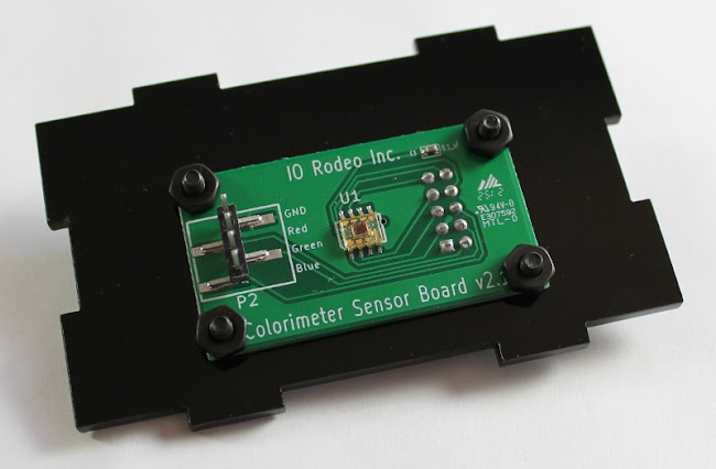
Step 6. Mount the Colorimeter Sensor Board onto the sensor mount passing the plastic 10-pin connector through the rectangular cutout (left and center images). Before securing in place ensure the correct orientation of the PCB as shown in the lower right image. Secure in place with the last four PCB screws and nuts.
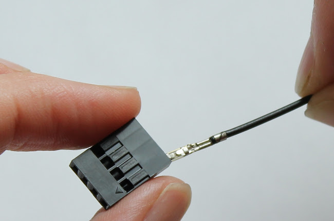
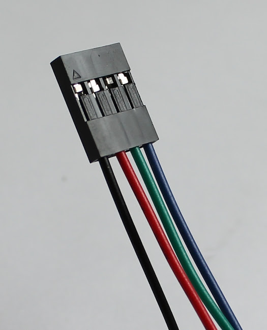
Step 7. From Bag B, take one of the black, plastic 4-pin connectors and the black pre-crimped wire. Locate the triangle marker on the housing which denotes Pin 1. Carefully push the black wire into the Pin 1 slot of the connector until it clicks into place. Next, insert the red wire into the Pin 2 slot of the connector, followed by the green wire (Pin 3 slot), and finally the blue wire (Pin 4 slot). Make sure all wires are held firmly in place by gently pulling on them. Do not put the connector on the other end of the wires at this point.
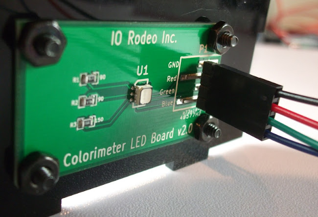
Step 8. Connect the assembled wires to the LED board (image below) so that the black wire is connected to the pin on the PCB labelled GND, the red wire to the pin labelled Red, the green wire to the pin labelled Green, and the blue wire to the pin labelled Blue. Thread the free ends of the four colored wires through the round hole in the divider wall.
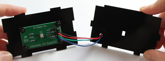
Step 9. Take the second 4-pin connector and, as before, insert the pre-crimped wires. Remember to first locate the triangular marker on the connector, and then insert the black wire into the slot corresponding to Pin 1, followed by the red (Pin 2 slot), green (Pin 3 slot) and blue (Pin 4 slot) wires. Finally, after ensuring that the cables are properly attached, connect this to the Colorimeter Sensor Board using the same pin-orientation as before (black wire to GND pin, red wire to Red pin, etc).
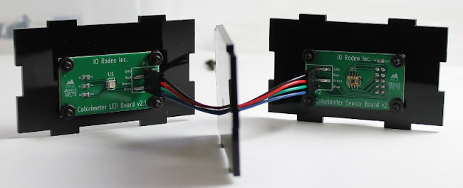
Step 10. Place the parts assembled in the previous step on the base plate taking note of the orientation. The sensor PCB and the divider wall should be on the side of the cuvette holder with the U-shaped cutout (left image). The cables may need to be adjusted to fit into the enclosure.
Step 11. Take the two side walls and insert them on the base plate so that all the corresponding tabs and slots match.
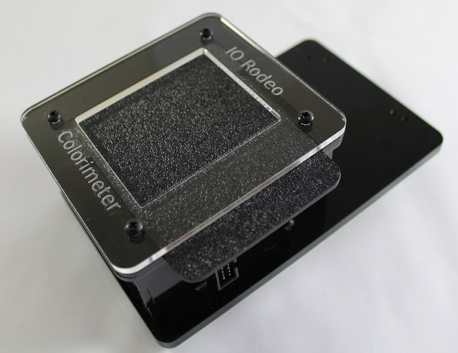
Step 12. Place the top plate on the enclosure ensuring that the tabs fit in the slots as shown in the Image below.
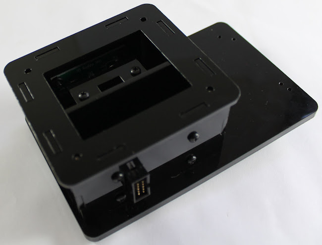
Step 13. Lay the outer slider and inner slider onto the top plate. Orient the parts as shown in the images below.
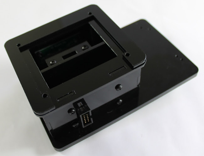
Step 14. Place the clear cover on the enclosure. Secure all the parts in place with the last four enclosure screws from Bag A.
You have now completed assembly of the colorimeter. In the next section you will mount the Arduino onto the base plate. If you will be using a TuxCase enclosure for the Arduino, skip down to the Instructions starting on Page 20.
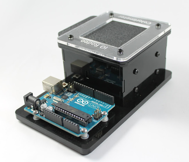
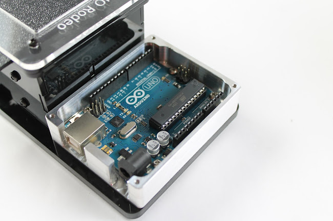
Assembly of Arduino onto base plate
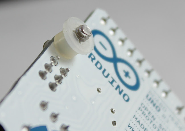
Step 1. To mount the Arduino Uno, take the bag of screws and plastic standoffs from Bag C. You do not need the 4 flat-head screws. Place one of the screws through one of the Arduino mount holes. On the other side place a plastic standoff and washer. The washer will hold the standoff in place while you work. Repeat for the remaining 3 mount-holes.
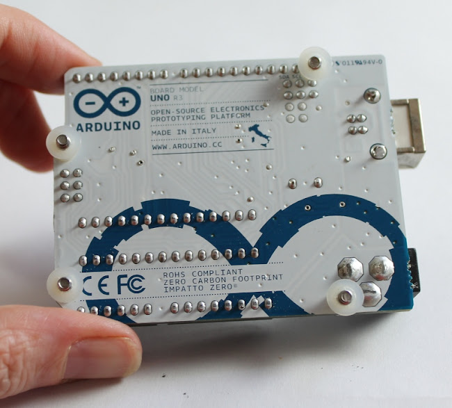
Step 2. Place the Arduino onto the base plate and line up the screws from the above step with the holes in the Arduino holes in the base plate. Screw them down into the base plate. Note: the screws will go partly into the base plate, not all the way through.
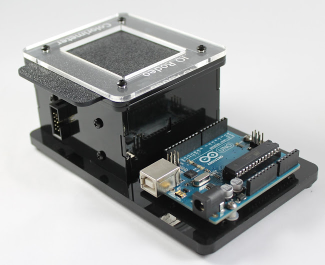
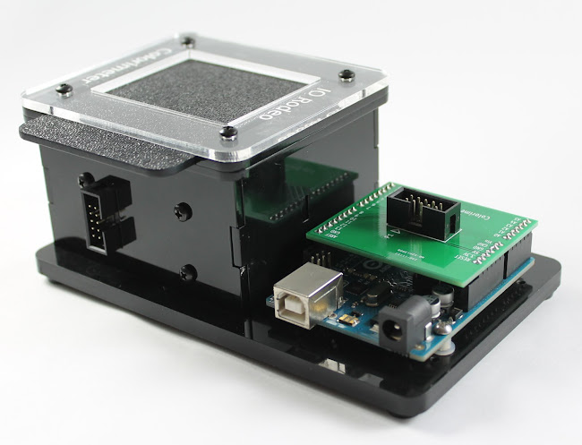
Step 3. Mount the colorimeter shield onto the Arduino board. There is only one orientation possible. Note that the shield pins are labelled on the silkscreen (white text) to match the label on the corresponding header on the Arduino board.
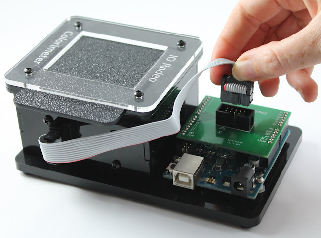
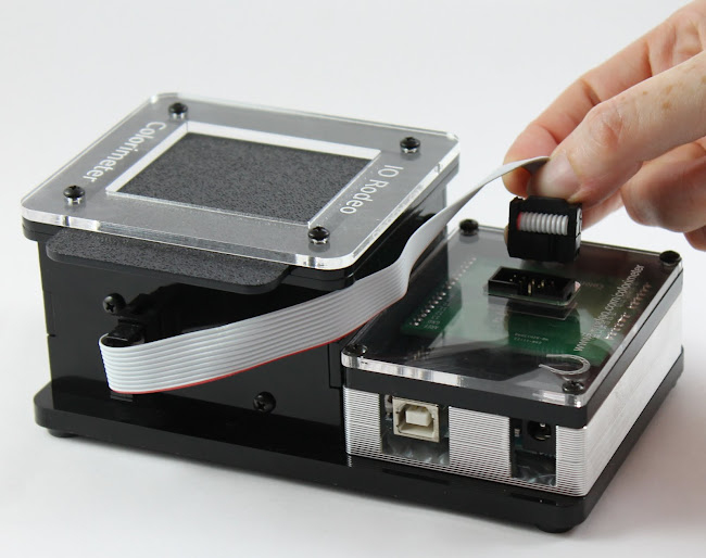
Step 4. Connect the ribbon cable to both the enclosure and the colorimeter shield. We have found it easier to connect the cable to the colorimeter first and then to the Arduino second.
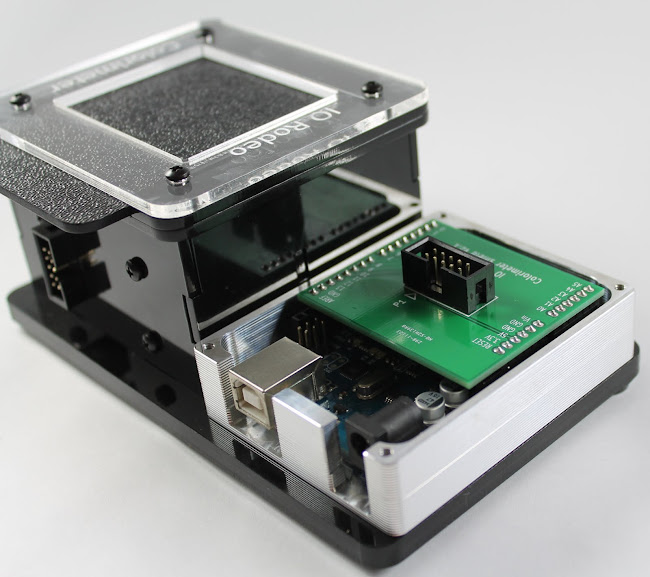
Optional: Assembly of Arduino with TuxCase
Step 1. To first mount the TuxCase onto the base plate, you will need the 4 flat-head screws from Bag C. Place the TuxCase on the base plate and line-up the four corner holes with the holes on the base plate. Fasten in place with the 4 flat-head screws.
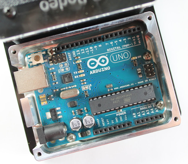
Step 2. Place the Arduino inside the TuxCase as shown in the Images below and fasten into the case using the 4 shorter (1/4”) screws that come with the TuxCase kit.
Step 3. Mount the colorimeter shield onto the Arduino board. There is only one orientation possible. Note that the shield pins are labelled on the silkscreen (white text) to match the label on the corresponding header on the Arduino board. Place the black acrylic spacer and the clear top onto the enclosure. Using the remaining 4 screws from the TuxCase kit, secure the top in place at the four corners.
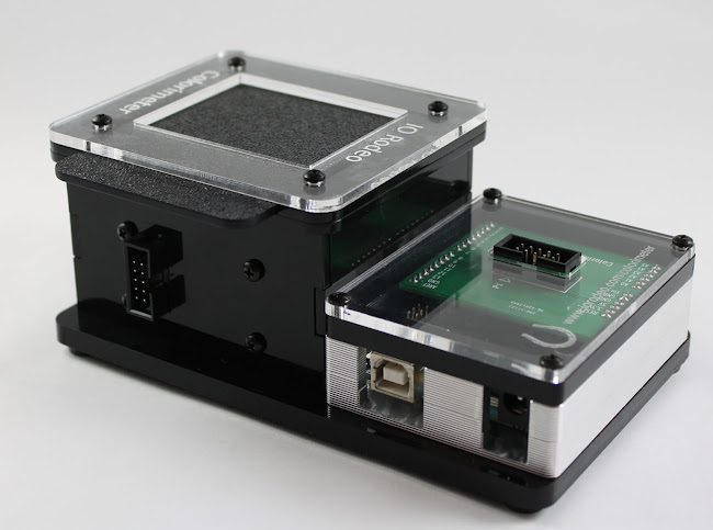
Step 4. Connect the ribbon cable to both the enclosure and the colorimeter shield. We have found it easier to connect the cable to the colorimeter first and then to the Arduino second.
Upgrading from original colorimeter hardware to the new design
For current users of the original colorimeter design (shown opposite) upgrading to the new single-piece design is very easy and only requires one additional piece of acrylic - the base plate - and some extra hardware. You can also choose to include the aluminum TuxCase Arduino enclosure. |
Upgrade 1: no TuxCase
- New base plate
- 6 x colorimeter enclosure screws (see hardware Bag A). These longer screws replace the original screws that mount the 6 standoffs to the acrylic base.
- 4 x Arduino screws, 4 x nylon standoffs and 4 x nylon washers (see hardware Bag C)
Upgrade 2: with TuxCase
- New base plate
- 6 x colorimeter enclosure screws (as in hardware Bag A). These longer screws replace the original screws that mount the 6 standoffs to the acrylic base.
- 4 x TuxCase screws (as in hardware Bag C)
- TuxCase kit - includes hardware (4 x 1/4" long 18-8 stainless screws for mounting Arduino into the TuxCase and 4 x 1/2" long 18-8 stainless screws for securing the clear acrylic top)
Step 1: Start by unscrewing and taking apart your colorimeter. Remove the standoffs and set aside the old base plate.
Step 2: With the new base plate and enclosure screws, follow the assembly steps in the User Manual to re-assemble the colorimeter.
Step 3: Follow the steps for either mounting the Arduino (kit 1) or mounting the TuxCase (kit 2).
Programming the Arduino with the Educational Colorimeter firmware[1]
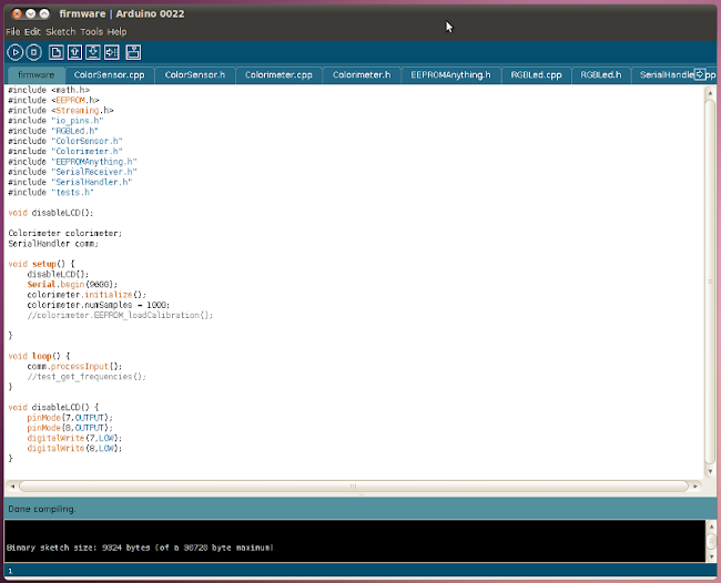
Download the Educational Colorimeter firmware from www.iorodeo.com/software/colorimeter onto your computer. Unzip the downloaded file to a known location. After unzipping, you should see an “colorimeter_firmware” folder containing the different files used by the firmware. Connect your Arduino board to the computer, start the Arduino IDE (installation instructions available at: http://arduino.cc/en/Guide/HomePage) and open the main firmware file “firmware.pde”. This file should compile without needing to download additional libraries. After selecting the Arduino board model, and the serial port it is using (under “Tools” menu of the Arduino IDE), upload the firmware to the board[2].
Educational Colorimeter software: data collection and analysis
Download the software for your choice of Operating System (Windows, Mac or Linux) from www.iorodeo.com/software/colorimeter. The files are provided as precompiled binaries so that they can be launched immediately after download (by double-clicking any of the 3 program files). For the more adventurous users, the source files are available at http://bitbucket.org/iorodeo/colorimeter/. The software suite we have developed for use with the Educational Colorimeter consists of 3 different programs. After download, unzip the “colorimeter_software_suite.zip” file onto a known location in your computer.
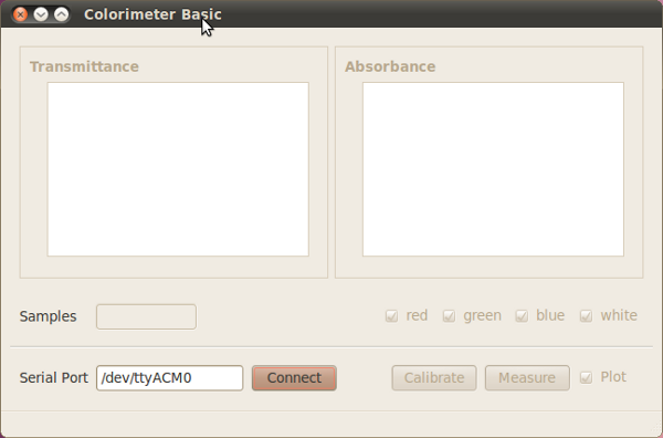
Colorimeter basic program
This program reports the Transmittance and Absorbance measured by the colorimeter for the wavelength(s) of light selected by the user. Instructions for using this software are as follows:
- Launch software: double-click on the colorimeter basic program icon, which can be found inside the previously downloaded “colorimeter_software_suite” folder;
- Establish connection: enter the serial port corresponding to your device in the program window and click on the “Connect” button in the lower left-hand side.
- Calibrate sensor: once connected to the hardware, you need to first take a calibration (“blank”) measurement to enable the “Measure” feature of the program. This needs to be done at least once (when you first start to use the program), but it can be done additionally at any time while taking measurements. Typically, a calibration measurement is carried out with a solution which does not contain any of the color you are interested in measuring. It is usually the liquid you used to dissolve or dilute your colored solution. In many cases, this liquid is water. As an example, if you are measuring the absorbance of blue food dye, you will use water to calibrate the color sensor. However, if you are carrying out a colorimetric assay, such as the ammonia assay in Lab 3, then you will calibrate against the assay solution developed with distilled water. In all cases, the steps are the same:
- Place a cuvette with water (or other “blank” solution) into the device;
- Click on “Calibrate”. The program will display a value of 1.00 for Transmittance and 0.00 for Absorbance on all color channels.
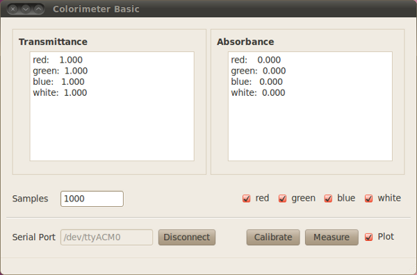
- Select LED: initially, all of the color channels are selected. You can deselect one or more of them at any time after calibration. The program will display values only for the selected color channels;
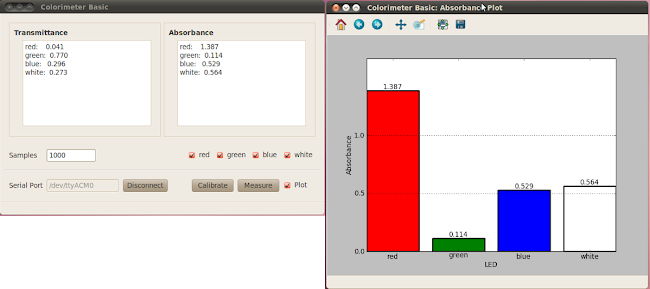
- Measure and plot data: place the cuvette, containing your sample, inside the enclosure and click “Measure”. The Transmittance and Absorbance text areas will display the measurements corresponding to the selected color channels. In addition, a second window will automatically open, displaying a bar graph of the measurements. If the bar graph is not needed for your measurements, uncheck the “Plot” checkbox.
Colorimeter plotting program
This program allows users to generate calibration curves that are typically used to find the concentration of a solution. Instructions for using this software are as follows:
- Launch software: double-click on the Educational Colorimeter Plotting program icon, which is inside the previously downloaded “colorimeter_software_suite” folder;
- Establish connection: enter the serial port corresponding to your device in the program window and click on the “Connect” button.
- Select LED: choose which LED to use from the options in the upper bar. Unlike the basic program, users can only select one LED for the measurements..
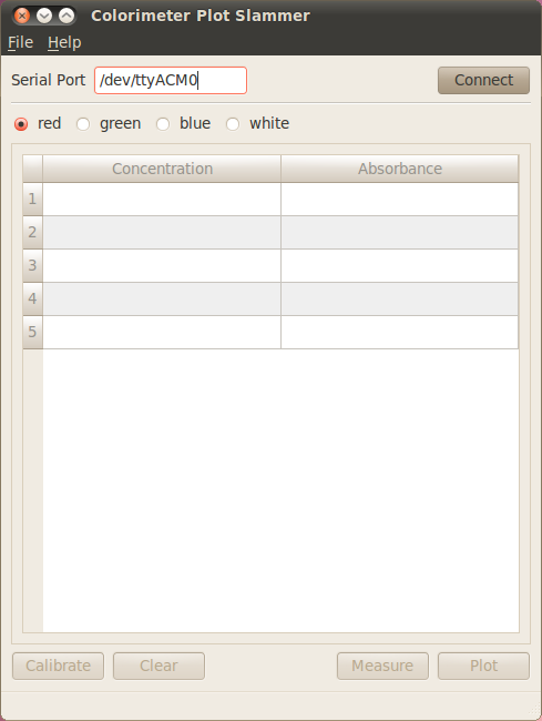
- Calibrate sensor: follow the calibration procedure described for the basic program. Note, that in this case, you should also measure the calibration solution (ie, sample with 0.00 Concentration) for including the zero data (Concentration, Absorbance) in your standard curve.
- Measure samples: place the cuvette, containing your sample, inside the enclosure and click “Measure”. The value for the absorbance measurement will be displayed in the first row of the table. You can either enter the concentration value, or skip ahead to the next measurement. Note that whereas the Concentration values are editable, the Absorbance measurements are not, as they correspond to readings from the sensor.
- Plot data: at any point after calibration, you can plot the data in the table by clicking “Plot”. A second window will automatically open, and display a scatter plot of the data.
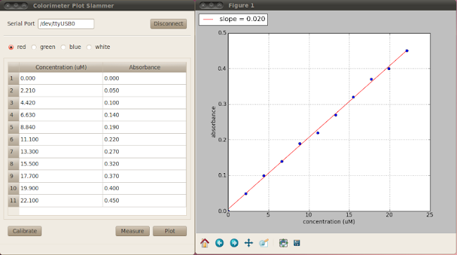
- Save data: at any point after calibration, you can save the data in the table to a standard, raw-text file. Using the “File -> Save” menu item at the top of the program window.
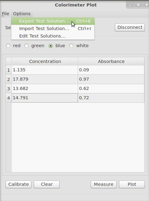
- Export standard curves: once you have your standard curve, you can export it for later use with the concentration program using the “Options-> Export Test Solution” menu item at the top of the program window . After exporting, this file will be automatically available for use with the concentration program.
Other features: Users can also clear data and load/import previously saved data files.
Colorimeter concentration program
This program measures the concentration of an unknown solution. Instructions for using this software are as follows:
- Launch software: double-click on the concentration program icon, which is inside the previously downloaded “colorimeter_software_suite” folder;
- Establish connection: enter the serial port corresponding to your device in the program window and click on the “Connect” button.
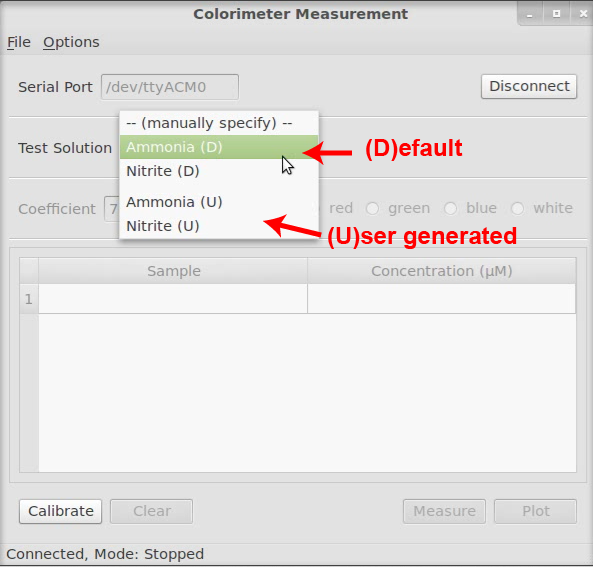
- Select standard curve: from the drop-down menu, select the standard curve corresponding to the solution you are going to be measuring. The menu contains both default and user generated standard curves. Optionally, the user may enter the coefficient and select the measurement LED manually.
- Calibrate sensor: follow the calibration procedure described for the basic program;
- Measure samples: place the cuvette, containing your sample, inside the enclosure and click “Measure”. The measured concentration values are displayed in these table. The user can edit the sample label.
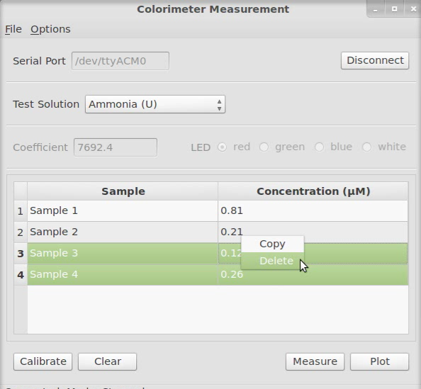
- Deleting data: even though the entries for Concentration are non-editable, you can select any number of rows, right-click anywhere on your selection, and select “Delete” to remove those entries from the table (image above). Note that the labels (Sample column) can be edited at any point.
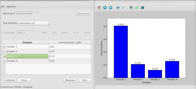
- Plotting data: if at least one Concentration value exists on the table, the data can be plotted by clicking the “Plot” button. On a separate window, a bar graph will display the data, in the same order as it is entered in the table. The bars will be labeled accordingly using the entries on the “Sample” column.
Lab 1: Introduction to Colorimetry
Background and Objectives
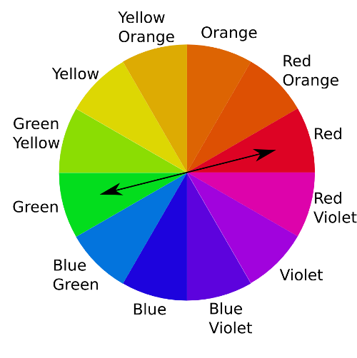
The visible light spectrum consists of a range of frequencies, each of which corresponds to a specific color. Any visible light that strikes an object and becomes reflected (or transmitted to our eyes) will contribute to the color appearance of that object. In the same way, the color of a solution is a direct result of the wavelengths of light absorbed by the solution. So, if a solution absorbs all of the frequencies of visible light except for the frequency associated with green light, then the object will appear green.
Complementary colors - Green and red are "complementary" colors, as shown on the color wheel below. A solution that absorbs mainly red light appears green and vice versa.
The objective of this lab is to build a colorimeter from electronic, mechanical, and software components, and use it to investigate how different colored solutions absorb different wavelengths of light.
Materials
- Educational Colorimeter kit
- Diluted food dyes - We have used FD&C red # 40, blue # 1 and yellow # 5 food dyes which can be found in most grocery stores. Dilute these dyes 10-fold before using in the lab. The green food dye is a mixture of the blue and yellow dyes.
- 5 x cuvettes (part of the Educational Colorimeter kit)
- 1 mL fixed volume pipette
- Water
Methods
This lab uses the Educational Colorimeter Basic program. Before starting the lab, download the software and review the operation of this program (details online and in your User’s Manual).
- Assemble the Educational Colorimeter enclosure, connect it to the Arduino board (using the colorimeter shield), and connect the board to the computer ensuring that it is running the colorimeter firmware. Use the instructions provided in the User’s Manual. This will take the majority of the lab to complete;
- Fill five cuvettes with 1 mL of water;
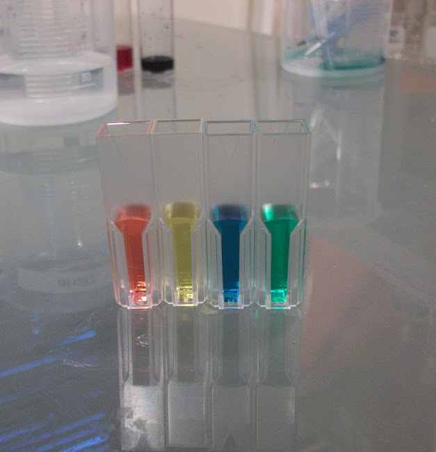
- Add 1 drop of diluted food dye (approximately 10 µL) to individual cuvettes. This will yield one cuvette with red dye, one with blue, one with green, and one with yellow. One cuvette should be left with just water for calibration. Mix the solutions by pipetting them up and down several times;
- Launch the colorimeter basic program on your computer;
- Place the cuvette with water in the colorimeter and click on calibrate. The display should now read 0.00 Absorbance (and 1.00 Transmittance) across all 4 color channel readings;
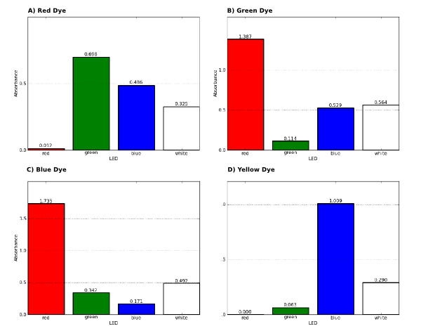
- Place the cuvette with red dye in the colorimeter and click on measure. Ensure that all color channels (Red, Green, and Blue) are selected in the program. Save the plot for later use if required;
- Repeat for the yellow, blue and green food dyes.
Sample Data
Lab 2: Beer's Law and Molar Extinction Coefficient
Background and Objectives
Colorimeters (and spectrophotometers) measure absorbance of light of a specific wavelength by a solution. Absorbance values can be used to determine the concentration of a chemical or biological molecule in a solution using the Beer-Lambert Law (also known as Beer’s Law). Beer’s Law states that absorbance of a sample depends on the molar concentration ( ), light path length in centimeters (
 ), and molar extinction coefficient (
 ) for the dissolved substance at the specified wavelength (λ)[3].
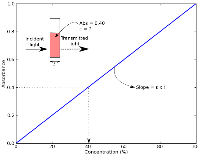
Beer-Lambert Law: 
An example of a Beer’s Law plot (concentration versus absorbance) is shown below. The slope of the graph (absorbance over concentration,/) equals the molar absorptivity coefficient, ε x . The objective of this lab is to calculate the molar extinction coefficients of three different dyes from their Beer’s Law plot.
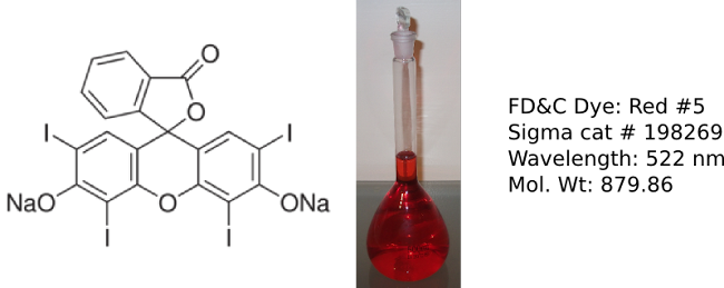
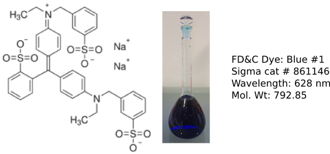
Food dyes are used to color a variety of food products such as sweets, cereal and sports drinks and are often used in high school and undergraduate labs[4]. The 3 dyes used in this lab were chosen as they absorb in the range of the colorimeter LED wavelengths.
Erythrosin B
Erioglaucine
Sunset Yellow

Materials
The following list of materials is required for this lab.
- Assembled Educational Colorimeter kit from Lab 1
- Powdered food dyes erythrosin B, erioglaucine and sunset yellow
- Analytical scale
- 3 x 250 mL volumetric flasks
- 15 x test tubes (>5 mL)
- 1 mL fixed volume pipette
- 16 x cuvettes
- Water
Methods
This lab uses the Educational Colorimeter Plotting program. Before starting the lab, download the software and review the operation of this program (details online and in your User’s Manual).
Step 1: Prepare 1 mM stock of dyes
- Erythrosin B (FW: 879.86): e.g. 0.218 g in 250 mL distilled water
- Erioglaucine (FW: 792.85): e.g. 0.198 g in 250 mL distilled water
- Sunset Yellow (FW:452.37): e.g. 0.113 g in 250 mL distilled water
Step 2: Preparation of standard curve
- Dilute the 1 mM stock solutions as shown in Table 1 using a 250 mL volumetric flask. Label these flasks working stock;
- For each of the 3 dyes, prepare a series of standard curve dilutions as shown in Table 2 using the test tubes. Label tubes #1-5 for each dye;
Step 3: Measure absorbance with the colorimeter and plot data
- Launch the colorimeter plotting program. Calibrate the device with a cuvette containing water as described in Lab 1.
- Starting with erythrosin B, measure the absorbance for each standard curve solution with the appropriate color channel[5], and enter the corresponding concentration in the program;
- Once all the samples are measured, click on the “Plot” button. Repeat measurements for erioglaucine and sunset yellow. Record values for the slope in Table 3.
Table 1: Preparation of working solutions
Dye | Volume of 1 mM stock | Concentration of working stock | Color channel/ wavelength |
Erythrosin B | 1 mL in 250 mL | 4.00 µM | Green/528 nm |
Erioglaucine | 2.5 mL in 250 mL | 10.00 µM | Red/625 nm |
Sunset Yellow | 10 mL in 250 mL | 40.00 µM | Blue/470 nm |
Table 2: Preparation of standard curves
Tube # | Volume of working stock | Erythrosin B | Erioglaucine | Sunset Yellow |
1 | 1 mL + 4 mL H2O | 0.8 µM | 2 µM | 8 µM |
2 | 2 mL + 3 mL H2O | 1.6 µM | 4 µM | 16 µM |
3 | 3 mL + 2 mL H2O | 2.4 µM | 6 µM | 24 µM |
4 | 4 mL + 1 mL H2O | 3.2 µM | 8 µM | 32 µM |
5 | 5 mL + 0 mL H2O | 4 µM | 10 µM | 40 µM |
Table 3: Molar extinction coefficient
Plotted Slope (µM vs. Abs) | Molar extinction coefficient (M-1 cm-1) | Reported value (Sigma spec sheets) | |
Erythrosin B | 0.056 | 56,000 at 528 nm |
(524-528 nm) |
Erioglaucine | 0.098 | 98,000 at 625 nm |
(627-637 nm) |
Sunset Yellow | 0.020 | 20,000 at 470 nm |
(479-485 nm) |

Sample Data
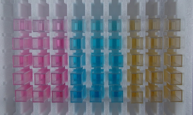
Fig 1: Image of cuvettes with 3 different food dye standard curves
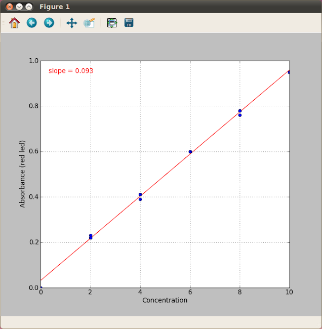
Fig 2: Sample data - Erioglaucine standard curve
Lab 3: Ammonia and nitrate measurements
Background and Objectives
Nitrification bacteria play an important role in the nitrogen cycle, oxidizing ammonia first to nitrite and finally to nitrate. Nitrification in nature is the result of actions of two groups of organisms:
(1) Nitrosomonas bacteria - ammonia-oxidizing bacteria convert ammonia to nitrite;
NH3 + O2 → NO2− + 3H+ + 2e−
(2) Nitrifying bacteria - nitrite-oxidizing bacteria convert nitrite to nitrate
NO2− + H2O → NO3− + 2H+ + 2e−
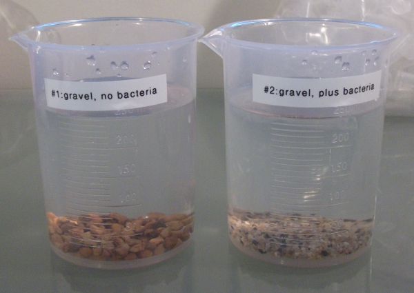
The objective of this lab is to monitor the levels of ammonia and nitrate over the course of 4 days in the presence of nitrification bacteria. Nitrification bacteria are widespread in soil and water and are found in highest numbers where considerable amounts of ammonia are present. In this lab, substrate (gravel) from an established aquarium will be used as the source of nitrification bacteria.
Colorimetric tests
Previously, in Labs 1 and 2, we used food dyes which are already colored. However, ammonia and nitrate are colorless in water. In this lab we will use colorimetric assays which yield a color only in the presence of ammonia or nitrate.
Ammonia - Salicylate test
The ammonia-salicylate method involves a three-step reaction sequence. The first reaction step involves the conversion of ammonia to monochloroamine by the addition of chlorine. The monochloroamine then reacts with salicylate to form 5-aminosalicylate. Oxidation of 5-aminosalicylate is carried out in the presence of a catalyst, nitroferricyanide, which results in the formation of indosalicylate, a blue-colored compound. The blue color is masked by the yellow color (from excess nitroprusside) yielding a green-colored solution that absorbs light at 650 nm. The intensity of the color is directly proportional to the ammonia concentration in the sample.
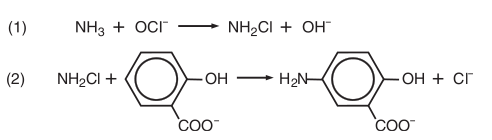
(1) Ammonia compounds are initially combined with hypochlorite to form monochloramine;
(2) Monochloramine reacts with salicylate to form 5-aminosalicylate.
Nitrate - Enzyme based assay
The assay for measuring nitrate is a 2-step process. First, nitrate in the sample is converted to nitrite enzymatically using nitrate reductase (NR). In the second step, nitrite is measured using Greiss test[6]. In the Greiss test, sulfanilamide reagent is converted to a diazonium salt by nitrite. The diazonium salt is then reacted with the reagent NED (N-1-napthylethylene diamine dihydrochloride) to form a colored azo dye which has a purple/magenta color that is measured at 520-550 nm (using the green LED).
Step 1) Nitrate reductase:
NO3- + NADH + H+ → NO2- + NAD + H2O
Step 2) Griess reaction:
Materials
- Labware: Beakers, volumetric flasks, graduated pipettes, test tubes, solution storage bottles; microfuge tubes;
- Store bought aquarium gravel (unused);
- Gravel from an established (and healthy) aquarium.
Chemicals and solutions
Chemical | Vendor | Cat # | Approx. Cost |
Sodium hydroxide | Carolina Biologicals | 889425 | $5.25 |
Sodium salicylate | Sigma | S2679-100G | $35.00 |
Sodium nitroferricyanide | Sigma | 228710-5G | $30.20 |
6% Sodium hypochloride | common household bleach available from most grocery and hardware stores. | $2.00 | |
Nitrate Reductase (2 Units) | NECi (Nitrate Elimination Company) | 800302 | $39.00 |
NADH | Sigma | 43420-100MG | $28.90 |
EDTA | Carolina Biologicals | 861780 | $16.25 |
Potassium phosphate (KH2PO4) | Sigma | P5655-100G | $21.50 |
Potassium hydroxide | Carolina Biologicals | 883485 | $5.25 |
Sulfanilamide | Sigma | S9251-100G | $33.70 |
3M Hydrochloric acid | Carolina Biologicals | 867861 | $6.75 |
NED (N-1-naphthylethylenedi-amine dihydrochloride) | Sigma | 33461-5G | $38.50 |
1,000 ppm ammonia | Scientific Strategies | 615-4RC | $17.82 |
10 ppm ammonia | Scientific Strategies | 5450-4RC | $16.55 |
10 ppm Nitrate standard | Scientific Strategies | 5456-4RC | $16.55 |
Distilled water | Most grocery stores | $2.00 |
Methods
This lab requires the use of both the Educational Colorimeter Plotting and Concentration programs. Using the “Export” functionality of the former, standard curves are generated for use in the latter. Before starting the lab, download the software and review the operation of these programs.
Day 0) Setting up the experiment and initial sample collection
- Transfer 1 mL of a 1,000 ppm ammonia stock to a 500 mL volumetric flask. Bring up to the mark using distilled water. This is your 2 ppm ammonia stock;
- Divide the 2 ppm solution into two beakers and label one as “Gravel” and another as “Gravel + Bacteria”.
- Take a scoop (25–50 g) of aquarium gravel from the store bought bag. Place in the beaker labelled “Gravel”.
- To obtain nitrification bacteria, remove an equivalent amount of gravel from an established aquarium as your source of nitrification bacteria. Place in the beaker labelled “Gravel + Bacteria” .
- Transfer 1.5 mL of sample to a clean microfuge tube for ammonia measurements.
- Transfer 1.0 mL of sample to a clean microfuge tube for nitrate measurements.
- Label these two samples as “T=0” (since they are taken at Day 0 of the experiment). Store them at –20°C.
- Repeat sampling every 24 hours for the following 4 days of the experiment, and label them “T=1”, …, “T=4”, respectively. You will collect a total of 10 samples (5 for ammonia, and 5 for nitrate measurements).
Day 2) Prepare solutions
Prepare the following solutions for making the ammonia and nitrate measurements. A list of the chemicals can be found in the Appendix (online).
1) Hypochlorite solution:
- Place 1 ml of bleach into a 100 mL volumetric flask and fill with 70 mL of DI water;
- Add 0.5 grams of NaOH and mix until dissolved;
- Fill flask to the 100 mL mark.
2) Salicylate/Catalyst solution:
- Place 10 g of sodium salicylate into a 100 mL volumetric flask and fill with 70 mL of DI water until dissolved.
- Add 0.04 grams of sodium nitroferricyanide and mix until dissolved.
- Add 0.5 grams NaOH to adjust the pH to the ~12.0 range.
- Fill flask to the 100 mL mark. Transfer solution into a dark, airtight glass bottle for maximum longevity. Due to limited storage life, prepare fresh solutions weekly.
3) 25 mM EDTA
- Dissolve 9.3g EDTA in 1L of distilled water.
4) Phosphate buffer (25 mM KH2PO4, 0.025 mM EDTA, pH 7.5)
- Dissolve 3.75 g of potassium phosphate (KH2PO4) and 1.4 g potassium hydroxide (KOH) in 800 mL of distilled water in a 1L volumetric flask
- Add 1 mL of 25 mM EDTA and fill to the mark
5) 2 units/mL nitrate reductase
- Add 1 mL of NECi proprietary enzyme diluent to 2 units of freeze-dried enzyme and reconstitute following the instructions supplied with the enzyme.
6) 1 mg/mL NADH
- Dissolve 0.1 g of NADH (FW=709.4) in 100 mL distilled water. Aliquot and store unused NADH in the freezer.
7) 1% sulfanilamide solution
- Weigh out 0.15g of sulfanilamide into a small amber bottle. Add 15 mL of 3M HCl.
8) 0.02% NED
- Weigh out 0.02 g of NED into an amber bottle. Add 100 mL of distilled water.
Day 3) Prepare ammonia standard curve
- Transfer 20 mL of the 10 ppm ammonia standard solution to a 100 mL volumetric flask. Fill flask to the 100 mL mark with distilled water and invert several times to mix. Label flask as 2.0 ppm ammonia.
- Label nine large test tubes #1-9. Pipette the indicated volumes of 2.0 ppm ammonia and distilled water into the test tubes as shown in the Table below.
Tube # | N Conc (ppm) | NH3 Conc (ppm) | NH3 Conc (µM) | Volume of 2.0 ppm ammonia (mL) | Volume of distilled water (mL) |
1 | 0.00 | 0.000 | 0.00 | 0.0 | 8.0 |
2 | 0.25 | 0.305 | 17.9 | 1.0 | 7.0 |
3 | 0.50 | 0.610 | 35.8 | 2.0 | 6.0 |
4 | 0.75 | 0.915 | 53.7 | 3.0 | 5.0 |
5 | 1.00 | 1.220 | 71.6 | 4.0 | 4.0 |
6 | 1.25 | 1.525 | 89.5 | 5.0 | 3.0 |
7 | 1.50 | 1.830 | 107.4 | 6.0 | 2.0 |
8 | 1.75 | 2.135 | 125.3 | 7.0 | 1.0 |
9 | 2.00 | 2.440 | 143.2 | 8.0 | 0.0 |
- Transfer 1 mL of each sample to be tested into a new test tube. Note: we recommend doing the measurements in triplicate.
- Add 250 µL of hypochlorite solution and mix
- Add 250 µL of salicylate/catalyst solution and mix
- Let tubes stand for 5-10 mins to develop color.
- Launch the Educational Colorimeter Plotting program, and select the Red color channel.
- Transfer the contents of Tube #1 (0.0 µM ammonia) into a cuvette, and use it for calibration.
- Before removing the calibration sample from the enclosure, click “Measure” (Absorbance value should be ~0.00).
- In the cell next to the measurement, enter the concentration value in µM (which in this case is 0.0).
- Transfer the contents back into the test tube. (It is good practice to rinse the cuvette with distilled water between samples)
- Transfer the next solution (Tube #2) into the cuvette, place it inside the enclosure, and click “Measure”.
- In the cell next to the measurement, enter the concentration value in µM.
- Repeat steps 11–13 for the remaining samples.
- After completing all measurements, and entering all concentration values, click “Plot” to graph your data. The points should roughly follow a linear trend (see sample graphs below).
- Using the file menu, go to “File>Export”, choose a filename for storing your sample curve (eg, student1_ammonia_sc), and click “OK”.
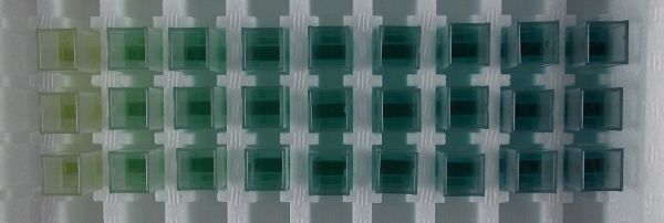
Fig 1: Image of cuvettes with ammonia standard curve in triplicate
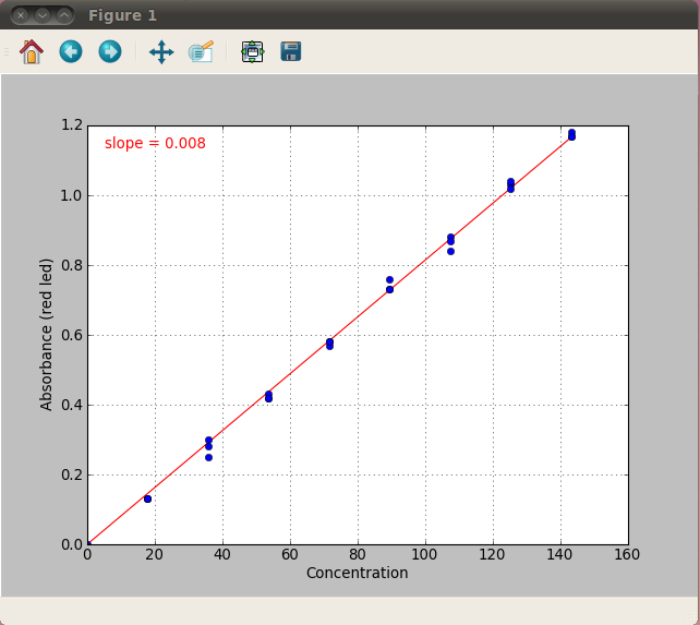
Fig 2: Sample ammonia standard curve
Day 4) Prepare nitrate standard curve
- Remove the NADH and nitrate reductase prepared in Step 2 from the freezer. Thaw the NADH. In a test tube, prepare a “10 x master mix” of enzyme, NADH and phosphate buffer as shown in the Table below.
Per sample | 10 x master mix | |
Phosphate buffer | 890 µL | 8.9 mL |
1 mg/mL NADH | 100 µL | 1 mL |
2 Units/mL Nitrate reductase | 10 µL | 0.1 mL |
Total Volume | 1000 µL | 10 mL |
- Label nine tubes #M1, M2, …, M9. To each tube transfer 1 mL of the master mix.
- To prepare the standard curve samples, label nine test tubes #1–9. Pipette the indicated volumes of 10 ppm nitrate standard and distilled water into these test tubes as shown in the Table below.
Tube # | N Conc (ppm) | NO3 Conc (ppm) | NO3 Conc (µM) | Volume of 10 ppm nitrate (mL) | Volume of distilled water (mL) |
1 | 0.0 | 0.00 | 0.00 | 0.0 | 8.0 |
2 | 1.25 | 5.537 | 89.25 | 1.0 | 7.0 |
3 | 2.50 | 11.075 | 178.5 | 2.0 | 6.0 |
4 | 3.75 | 16.613 | 267.75 | 3.0 | 5.0 |
5 | 5.00 | 22.15 | 357 | 4.0 | 4.0 |
6 | 6.25 | 27.688 | 446.25 | 5.0 | 3.0 |
7 | 7.50 | 33.225 | 535.5 | 6.0 | 2.0 |
8 | 8.75 | 38.763 | 624.75 | 7.0 | 1.0 |
9 | 10.00 | 44.3 | 714 | 8.0 | 0.0 |
- Add 50 µL of each standard curve sample to the corresponding tube containing the master mix (eg, from tube #1 to tube #M1, etc.). Mix thoroughly and incubate for 20–30 minutes.
- Add 500 µL of 1% sulfanimide to each tube and mix
- Add 500 µL of 0.02% NED to each tube and mix.
- Launch the Educational Colorimeter Plotting program, and select the Green color channel.
- Transfer the contents of Tube #M1 (0 ppm nitrate) into a cuvette, and use it for calibration.
- Before removing the calibration sample from the enclosure, click “Measure” (Absorbance value should be ~0.00).
- In the cell next to the measurement, enter the concentration value in µM (which in this case is 0.0).
- Transfer the contents back into the test tube. (It is good practice to rinse the cuvette with distilled water between samples)
- Transfer the next solution (Tube #M2) into the cuvette, place it inside the enclosure, and click “Measure”.
- In the cell next to the measurement, enter the concentration value in µM.
- Repeat steps 11–13 for the remaining samples.
- After completing all measurements, and entering all concentration values, click “Plot” to graph your data.
- Using the options menu, go to “Options>Export”, choose a filename for storing your sample curve (eg, student1_nitrate_sc), and click “OK”.
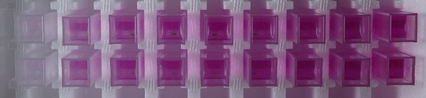
Fig 3: Image of cuvettes with nitrate standard curve in duplicate
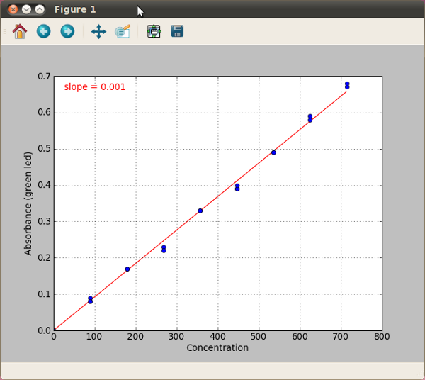
Figure 4: Sample nitrate standard curve
Day 5) Measure nitrate and ammonia in samples
Take your last sample from the experiment (“T=4”). Remove from the freezer the samples collected on previous days (“T=0”, …, “T=3”) and thaw.
- Process all 10 samples (5 for nitrate, and 5 for ammonia measurements) the same way as you did for generating the standard curves on Days 3 and 4. Don’t forget to also process a distilled water sample for calibration.
- Once you have the samples ready for measurement, open the Educational Colorimeter Concentration program.
- Starting with ammonia, select the standard curve generated on Day 3 from the drop down list (eg, “student1_ammonia_sc”). Note that the Red color channel will be automatically selected.
- Calibrate the colorimeter with the 0 µM ammonia control, and measure all of your ammonia samples. Label the corresponding measurements as “Day 0”, …, “Day 4”.
- Once you have finished click the “Plot” button. Save the displayed graph.
- Repeat steps above for nitrate. Select the standard curve generated on Day 4 from the drop down list. Note the Green color channel will be automatically selected.
- The two bar graphs should follow a linear trend as a function of time (see sample data below).
Sample Data
A) Ammonia concentration (uM) B) Nitrate Concentration (uM)
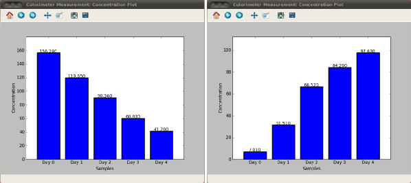
Fig 5: Final experimental data showing ammonia decreasing and nitrate increasing as a result of nitrification bacteria.
Day | Ammonia (uM) | Nitrate (uM) |
0 | 156.240 | 0.87 |
1 | 147.27 | 1.79 |
2 | 146.18 | 0.63 |
3 | 122.70 | 1.77 |
4 | 155.21 | 0.00 |
Table: Ammonia and nitrate concentration in the control sample (no nitrification bacteria).
[1] Note: If you received a pre-programmed Arduino with your colorimeter kit, then you can skip this step.
[2] More detailed instructions for using the Arduino IDE can be found at: http://arduino.cc/en/Guide/Environment
[3] Path length (distance that light travels through the solution) is determined by the cuvette that the sample is placed in. Most colorimeters and spectrophotometers, including the one in this kit, use cuvettes with a path length of 1 cm. Molar extinction coefficient is a measure of how strongly a substance absorbs light at a particular wavelength, and is usually represented by the unit M-1 cm-1 or L mol-1 cm-1.
[4] For example: Sigman and Wheeler 2004, J. Chemical Education 81 (10): 1475-1478; Henary and Russell, 2007, J. Chemical Education 84 (3) 480-482.
[5] To determine which color channel to use, measure absorbance at all 3 wavelengths as described in Lab 1.
[6] Developed by Peter Griess in 1879, this standard test is widely used to detect nitrites.