Lab 1 – Part 1
Supplementary Worksheet
ENGR 1282.02H
Spring, 2016
Dip Patel
DMG - 12:40pm
Date of Submission: 2/26/16
Coarse Mesh:
- Insert screen shot of your goals plot below:
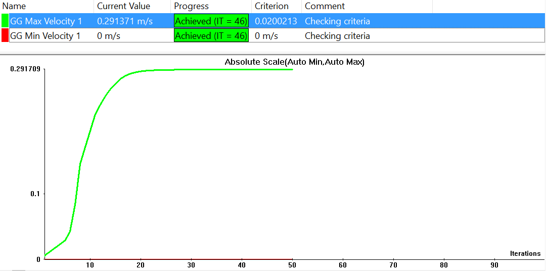
Figure 1: Goals plot after 50 iterations.
- Insert screen shot of your pressure contour surface plot below:
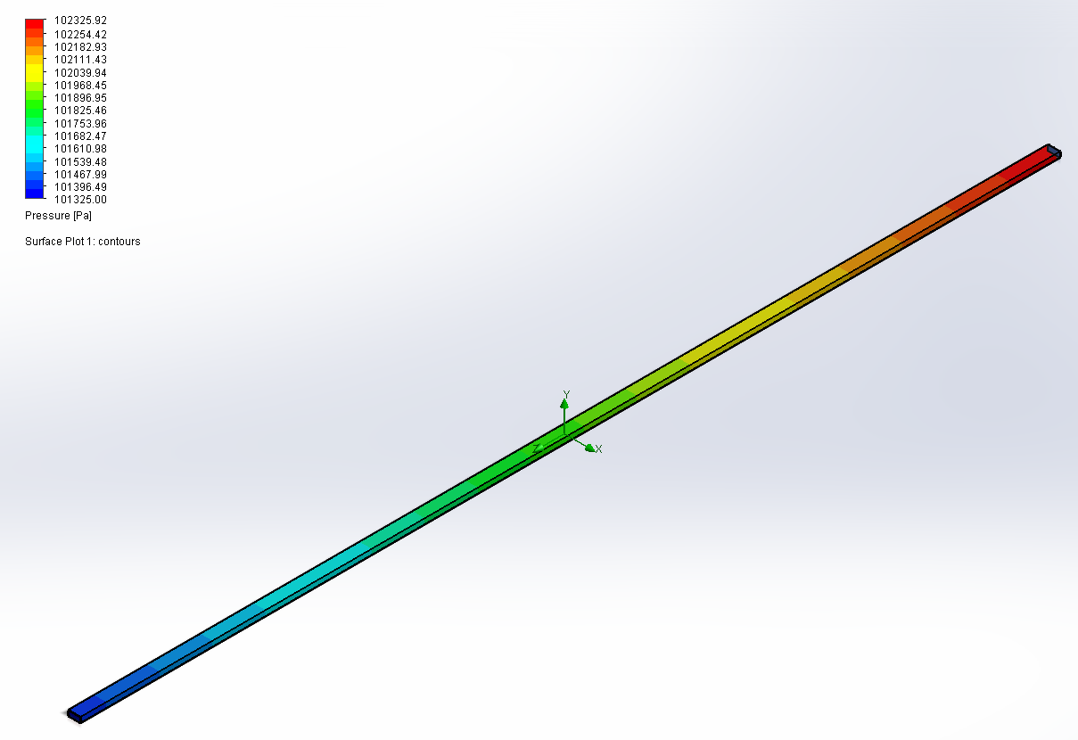
Figure 2: Contour surface plot.
- Insert screen shot of your Velocity Contours (z = 0.010 m) below:

Figure 3: Velocity contour at 0.010m.
- Insert a screen shot of your Velocity Vectors (z = 0.010 m) below:
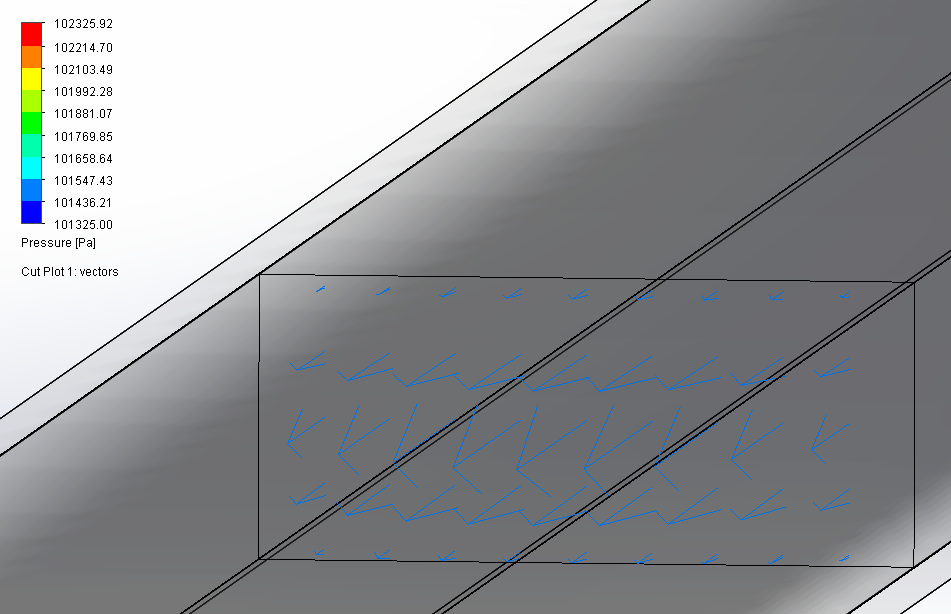
Figure 4: Velocity vectors.
- Insert a screen shot of your Flow Trajectories below:
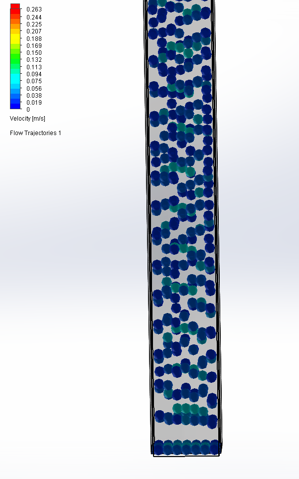
Figure 5: Flow Trajectories.
Fine Mesh:
- Insert a screen shot of your Goals Plot below:
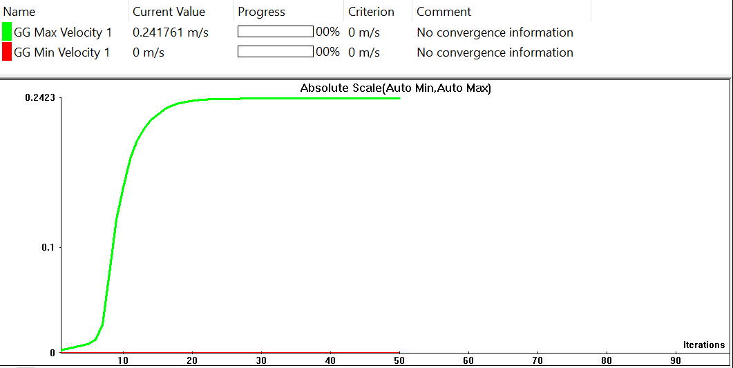
Figure 6: Fine Mesh Goals Plot.
- Insert screen shots of your 2-D velocity Contours below (z = 0.010m, -0.01240m, -0.01245m, -0.01250m, last 3 can be combined in one screenshot):
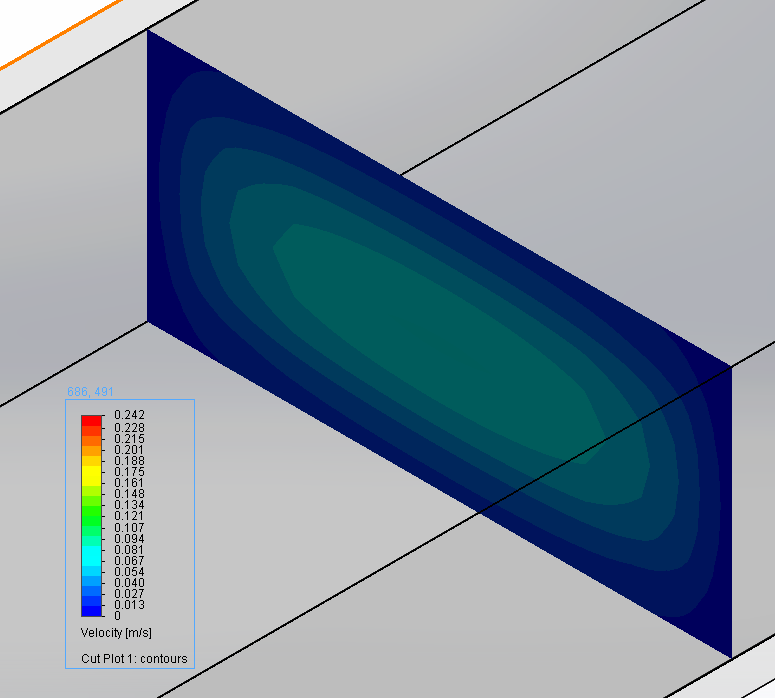
Figure 7: Velocity Contours at z = 0.010m.

Figure 8: Entrance effects contour plot.
- Insert a screen shot of your 3-D Velocity Contours below:
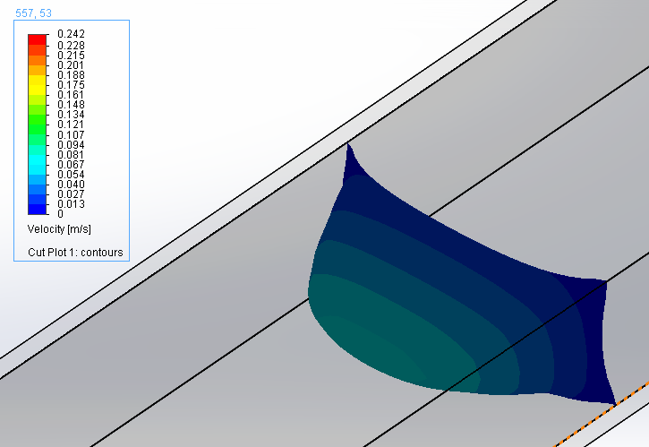
Figure 9: 3D Velocity Contours.
- Insert a screen shot of your Sheer Stress Contours below:

Figure 10: Shear stress contours.
- Discuss the flow profiles you achieved in this part of the lab. Are the results similar to what you would expect based on your knowledge of fluid mechanics? Why or why not? Consider laminar vs. turbulent flow, the no-slip condition, as well as any other concepts you think are important.
Yes, the results of this simulation are similar to what would be expected with prior knowledge of fluid dynamics. The fine mesh model had laminar flow and the no-slip condition at the boundary, which is visible on the velocity contours as a velocity of zero at the walls, and on the goals plot as a minimum velocity of zero. The 3D model of velocity proved the parabolic shape of velocity as predicted by the fluid mechanics equations.
- Discuss the differences you see between the results of the coarse and fine meshes. How do the flow velocities and profiles compare? Which mesh seems to do a better job of replicating the flow profile we would expect in the channel? (What known condition does one of the meshes violate, based on the flow profile produced?)
In the coarse mesh model, the smooth, parabolic shape of the velocity was not cleanly observed in the velocity contour, however in the fine mesh model it was. The fine mesh did a better job of replicating the flow profile expected as the 3D contour was parabolic in nature and observed the no-slip condition. The coarse model was not completely parabolic and did not observe the no slip condition.
- Based on the results from this part of the lab, how important is establishing a quality mesh before running your flow simulation? What could happen if the mesh is too coarse? What drawbacks might be present when using a fine mesh compared to a course mesh?
It is very significant to establish a quality, fine mesh in order to properly conduct the experiments. If the mesh is too coarse, the no-slip condition at the walls will not be observed and the whole experiment will fail. A potential drawback of using a fine mesh is the time/resources needed to fabricate such a mesh.
- After completing this part of the lab, how do you plan to assign a proper mesh for your custom chip design?
The finer the better. However, not too fine as to waste materials and time during fabrication. The whole point is to get the mesh to observe the no-slip condition. If that is met, then we have a good mesh.