Working with Mid-Ocean Ridge Features
Authors: Sabin Zahirovic, Serena Yeung, and James Egan
Updated for GPlates 2.2 and the reconstructions of Müller et al. (2019) by Behnam Sadeghi and Christopher Alfonso
EarthByte Research Group, School of Geosciences, The University of Sydney, Australia
Working with Mid-Ocean Ridge Features
Exercise 1 – Loading data and creating a MOR feature
Exercise 2 – Incorporating a new MOR feature into an existing plate polygon dataset
Extending a new MOR to intersect with existing plate boundaries
Aim
The aim of this tutorial is to teach the user how to (1) interactively create a new mid-ocean ridge (MOR) feature and (2) link it to existing adjacent plates in order for the MOR to reconstruct correctly through time.
Background
GPlates allows you to interactively create features (see Tutorial 1.5 Creating Features) such as subduction zones or volcanoes. When creating a MOR feature, its motion relative to the two adjacent plates is able to be automatically calculated by GPlates using half stage rotations (version3). Previously, GPlates could not easily handle generating MOR motions on the fly – and so the original continuously closing polygons have half stage rotations (version3) that were manually calculated.
We will go through the steps of how to interactively create a MOR and attach it to two adjacent plates so that it reconstructs correctly through time. We will also demonstrate how to incorporate a newly created MOR feature into an existing plate polygon dataset. Note that this is only a generalised tutorial designed to teach the user the basics of creating and working with MOR features.
Included files
Click here to download the data bundle for this tutorial.
The tutorial dataset includes the following files:
- Coastlines:Muller_etal_2019_Global_Coastlines.gpmlz
- Rotation model: Muller_etal_2019_CombinedRotations.rot
- Plate boundaries: Muller_etal_2019_PlateBoundaries_DeformingNetworks.gpmlz
This tutorial dataset is compatible with GPlates 2.2.
Exercise 1 – Loading data and creating a MOR feature
- Open GPlates and load the included tutorial dataset using Open Feature Collection. This dataset (Figure 1) includes the coastlines, plate boundaries, and rotations from Müller et al. (2019).
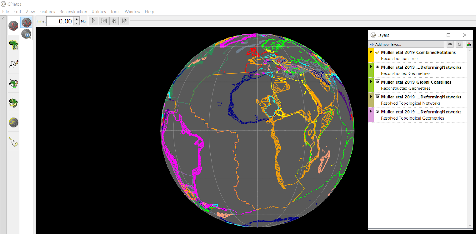
Figure 1. GPlates with the Müller et al (2019) datasets loaded.
- Click and drag the purple Resolved Topological Geometries layer (Muller_etal_2019_PlateBoundaries_DeformingNetworks) to the top of the Layers window, and hide the brown Resolved Topological Networks layer by clicking on the eye symbol (Figure 2).
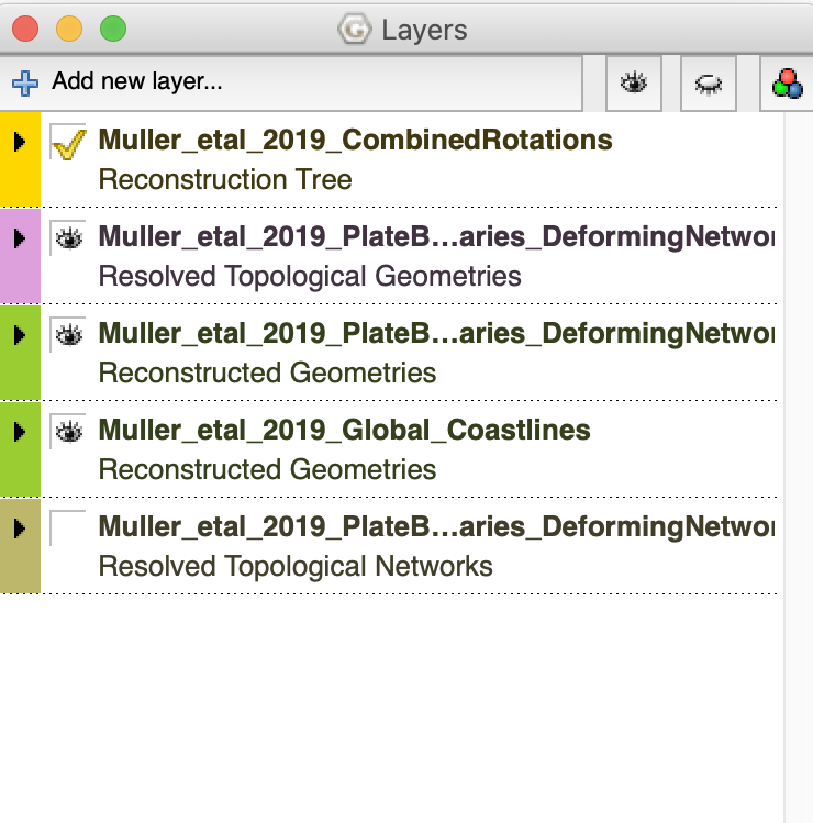
Figure 2. Click and drag the Resolved Topological Geometries layer (coloured purple) to the top of the list in the Layers window. Hide the Resolved Topological Networks layer.
It is suggested that the colouring for this dataset is changed to black (or any other easily-visible colour) to help identify these plate boundaries from the isochron file.
- Under the ‘Features’ menu, click ‘Manage Colouring’. Select the purple plate boundary topologies layer for recolouring, and under ‘Single Colour’, select the colour black (Figure 3).
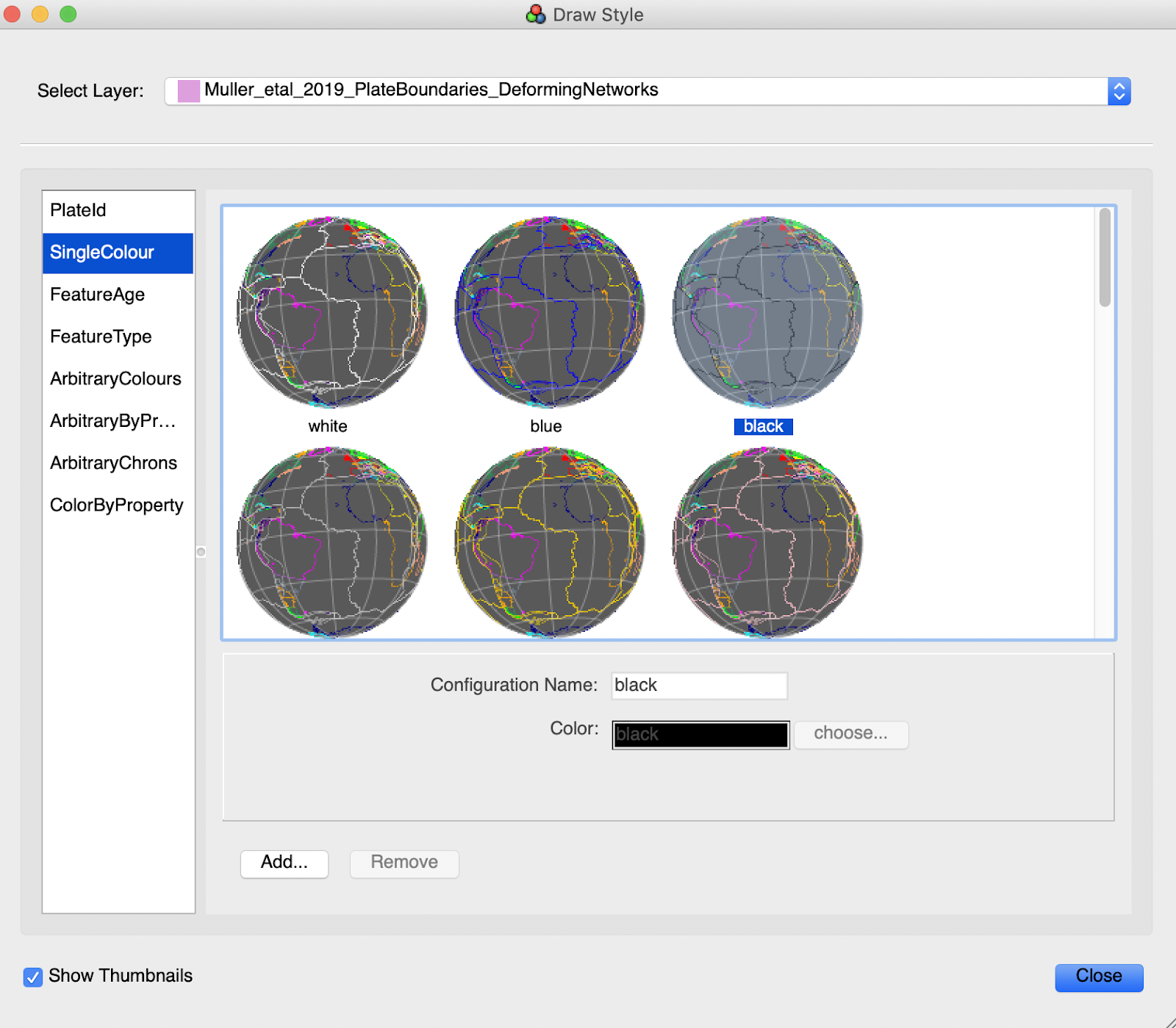
Figure 3. Recolour the plate boundary topologies layer black in the Manage Colouring window.
We will now interactively construct a new MOR feature. For this example, we will create a new MOR in the Atlantic Ocean, between South America and Africa, which exists between 60 and 20 Ma. For example’s sake, we will disregard the existing South America-Africa MOR, visible in black, and draw our new MOR on top of it.
- Reconstruct to 60 Ma and focus on the Atlantic Ocean (Figure 4).
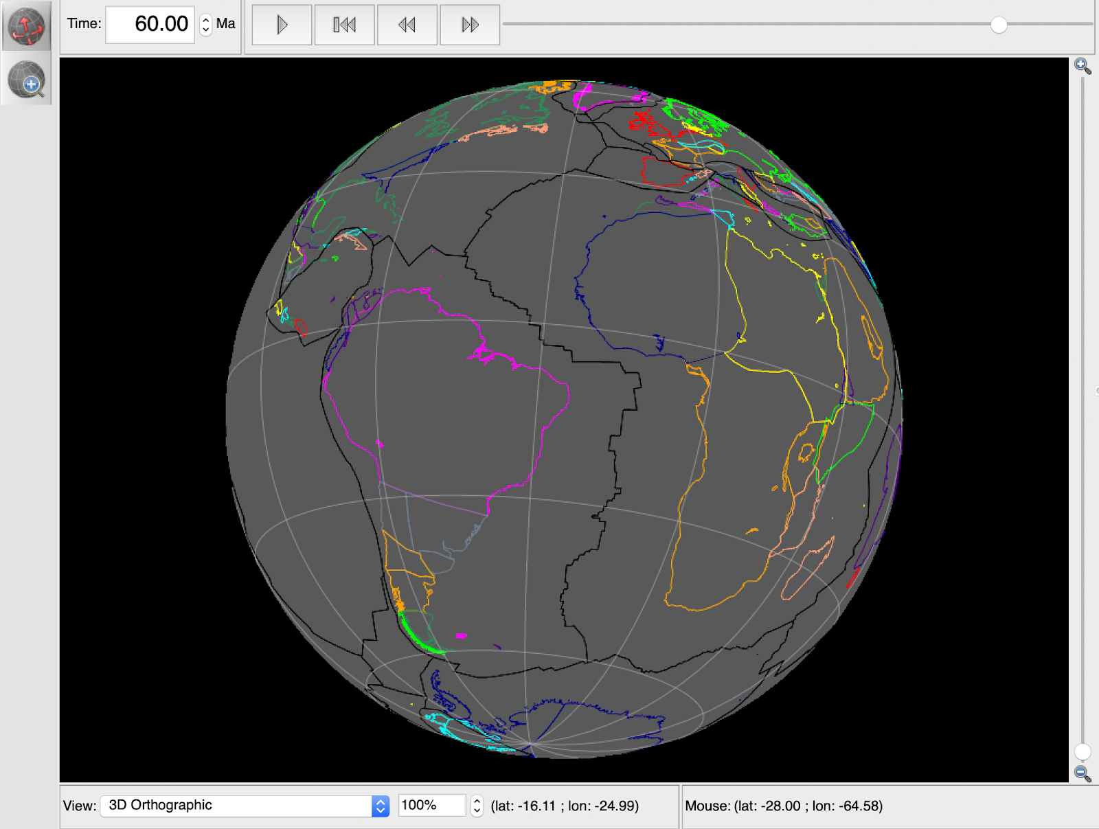
Figure 4. The Atlantic Ocean, Africa and South America reconstructed at 60 Ma.
In this example we will plot a fairly random MOR for the purposes of showing how to reconstruct it correctly through time. It does not have to intersect any existing plate boundaries, but this idea will come into play in Exercise 2 when we have to incorporate a MOR into an existing plate polygon dataset.
- Under the ‘Digitisation’ icon on the left, select ‘Digitise new polyline Geometry L’. You can now plot individual points on the main GPlates window by simply clicking the desired location. Digitise a line which roughly follows the existing MOR (Figure 5).

GPlates will automatically connect your series of plotted points in a ‘join-the-dots’ fashion to form a complete line coloured white (Figure 5). Notice that the coordinates of your points will appear in the ‘New Geometry’ window to the right of the GPlates main window. If you make a mistake in the location of your plotted point, use the keyboard command Ctrl-Z to undo the action.
- Once the line is complete, click the ‘Create Feature’ button on the right hand side of the GPlates main window to specify the properties of your newly created line (Figure 5).
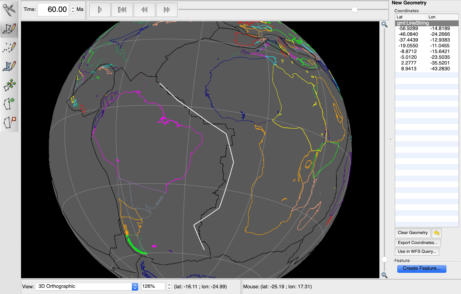
Figure 5. A digitised line (shown in white) plotted using the ‘Digitise new polyline feature’ tool. Click the highlighted ‘Create Feature’ button to specify the properties of the newly created line.
- In the first ‘Create Feature’ window, select the ‘MidOceanRidge’ feature type from the list, and click Next (Figure 6).
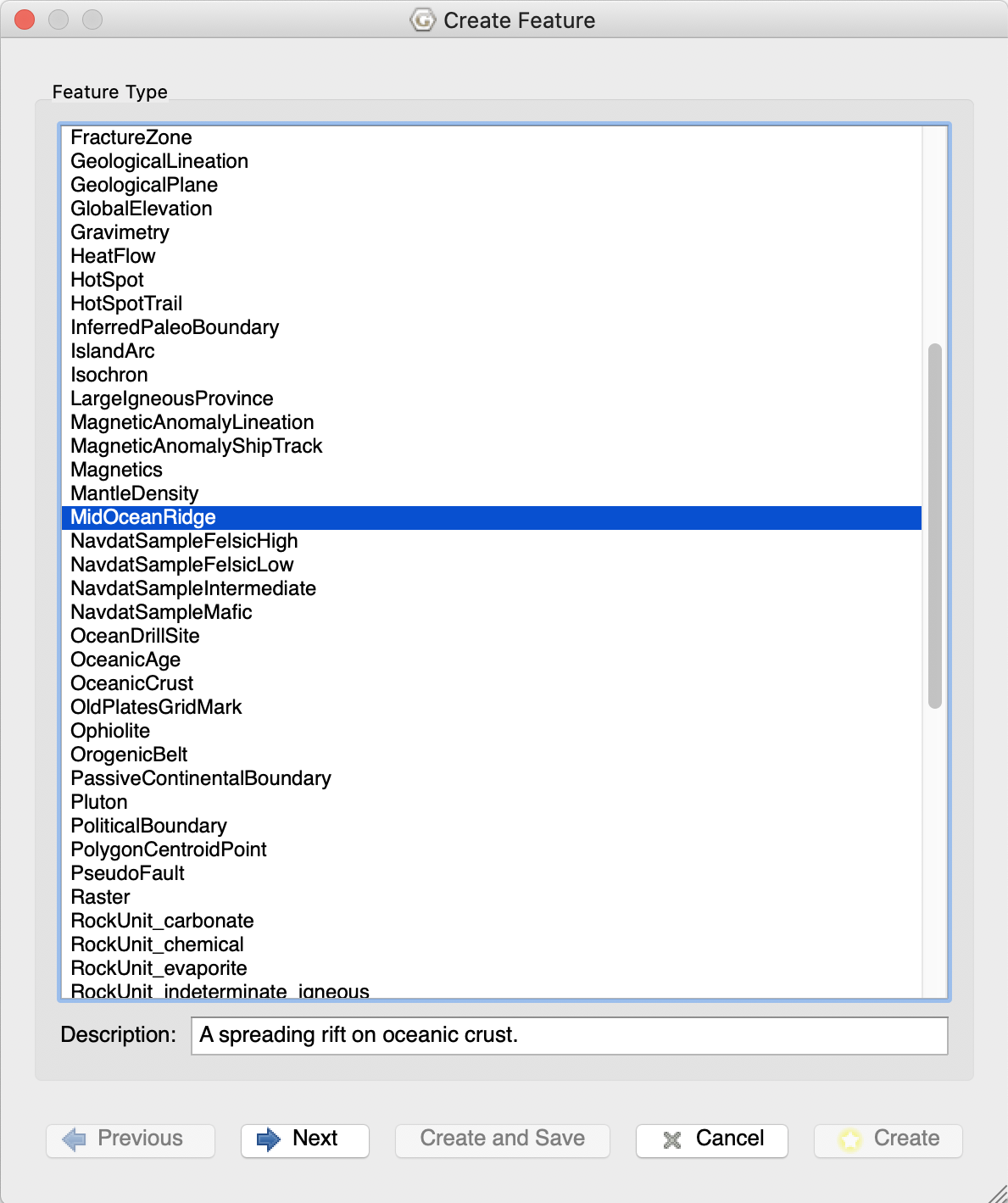
Figure 6. The first ‘Create Feature’ window with the feature type ‘MidOceanRidge’ selected.
- In the second ‘Create Feature’ window, feature properties such as the time of appearance and disappearance, file name and reconstruction method are able to be specified (Figure 7).
- Keep the default Geometry Property ‘Centre line’, as well as the Reconstruction Method: ‘Half stage rotation version3’.
- Specify the Left and Right Plate IDs – these are the conjugate Plate IDs.
For this example, these are 201 and 701 representing the South American (SAM) and African plates, respectively. Since our MOR feature doesn’t intersect any plate boundaries, the choice of conjugate Plate IDs is crucial in order for GPlates to correctly calculate the motion of the MOR through time. However, generally it does not matter which you decide is the left or right Plate ID as GPlates figures out the rest on its own.
- Specify the Begin time as 60 Ma (i.e., the appearance time of the MOR), the End time as 20 Ma (i.e., the disappearance time of the MOR) and the Name, and click Next (Figure 7).
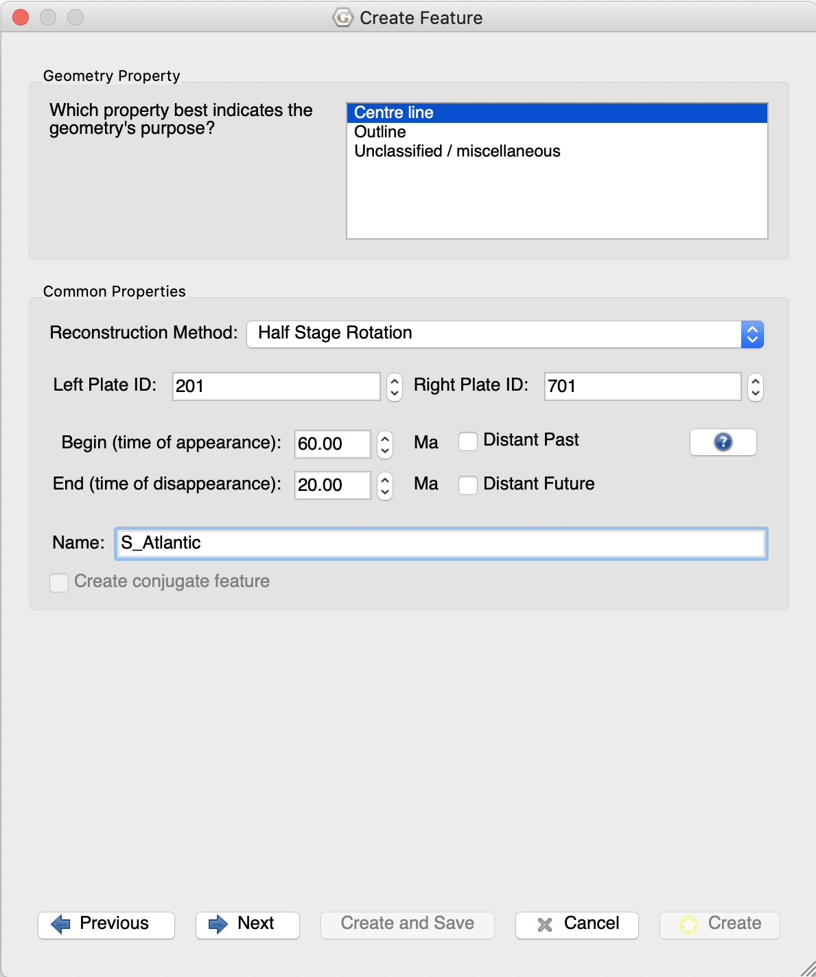
Figure 7. The second ‘Create Feature’ window where the reconstruction method, left and right Plate IDs, begin/end time and filename of the new MOR feature can be specified.
This opens up the third ‘Create Feature’ window which summarises the existing properties you have specified and any extra properties that are available to you.
- We will not change any more properties, so click Next, and Next again.
- In the fourth ‘Create Feature’ window select the plate boundaries dataset to save your new MOR to, and click Create (Figure 8).
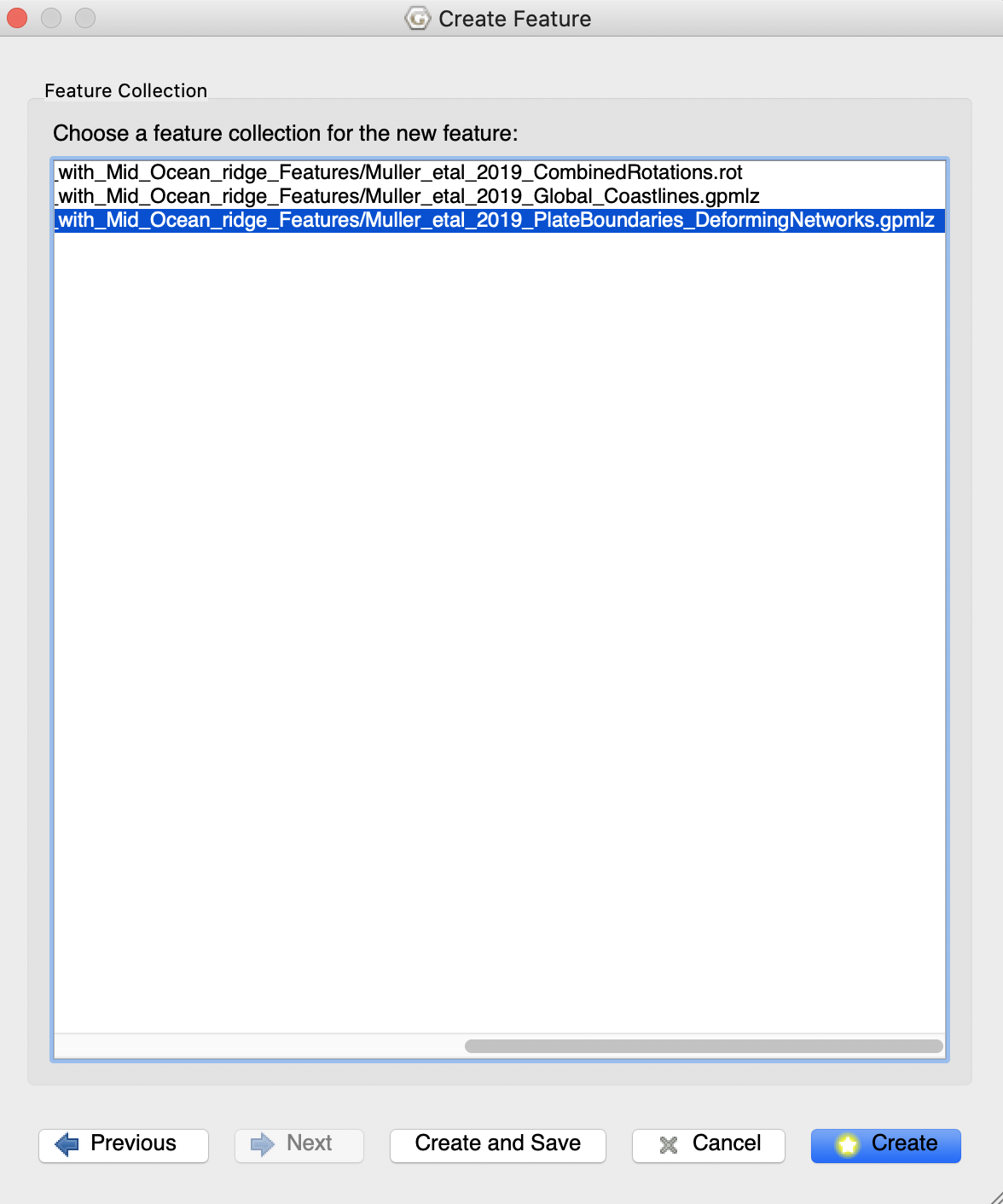
Figure 8. Select the plate boundaries dataset and click Create.
You will then be taken back to the main GPlates window.
- Select the new MOR using the ‘Choose Feature’ tool under the ‘Feature Inspection’ icon and click on the feature you have just created. All the properties that you have specified earlier will be shown in the adjacent windows (Figure 9).
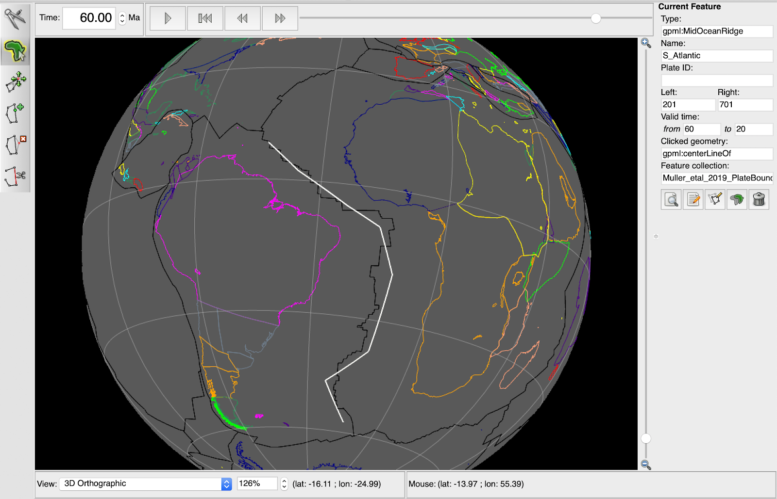
Figure 9. Use the ‘Choose Feature’ tool to inspect our newly created MOR and view the properties specified earlier.
Additionally, if you reconstruct forward in time, you will see your new MOR reconstructing correctly. Notice that after 20 Ma, the MOR ridge will disappear as we have specified. You have now learnt how to create a mid-ocean ridge feature in GPlates!
Exercise 2 – Incorporating a new MOR feature into an existing plate polygon dataset
We will now interactively construct a MOR feature with the intention of replacing an existing MOR. This requires the user to ensure the new MOR geometry intersects with pre-existing plate boundaries so that it can replace an old MOR. The user then has to delete the old MOR, and manually edit existing topologies to insert the new plate boundary. When deleting a MOR, the user must fix at least two polygons at any one time. That is because the old MOR formed the mutual boundary between two polygons.
Users must also take care to correct any other polygon artefacts they may have introduced by deleting the old redundant MOR. GPlates does not automatically detect polygon artefacts, so a careful interactive reconstruction in GPlates through time is required to ensure polygon closure without gaps, overlaps or “rubber-banding” artefacts.
For this example, we will again create a new MOR in the Atlantic Ocean adjacent to the existing South America-Africa MOR, which exists between 60 and 20 Ma.
- For the purposes of clarity, delete the MOR which was created in Exercise 1 by selecting it using the ‘Choose Feature’ tool and either tapping Delete on the keyboard, or clicking the trash bin ‘Delete Feature’ icon on the right-hand interface.
- Reconstruct to 60 Ma and focus on the black MOR between at the junction of the South American (SAM) Plate and the African Plate (Figure 10).

Figure 10. The Atlantic Ocean, Africa and South America reconstructed at 60 Ma, centred on the South America-Africa MOR.
- Under the ‘Digitisation’ icon on the left, select ‘Digitise new polyline geometry’.
- As in Exercise 1, plot a series of points which span the length of the existing South America-Africa MOR (Figure 11). Note that your new MOR geometry must intersect the pre-existing plate boundaries of the two conjugate plates (SAM and Africa). Again if you plot an incorrect point, use the keyboard command Ctrl-Z to undo the action. The Appendix will detail how to extend a new MOR to intersect with existing boundaries if it doesn’t already.
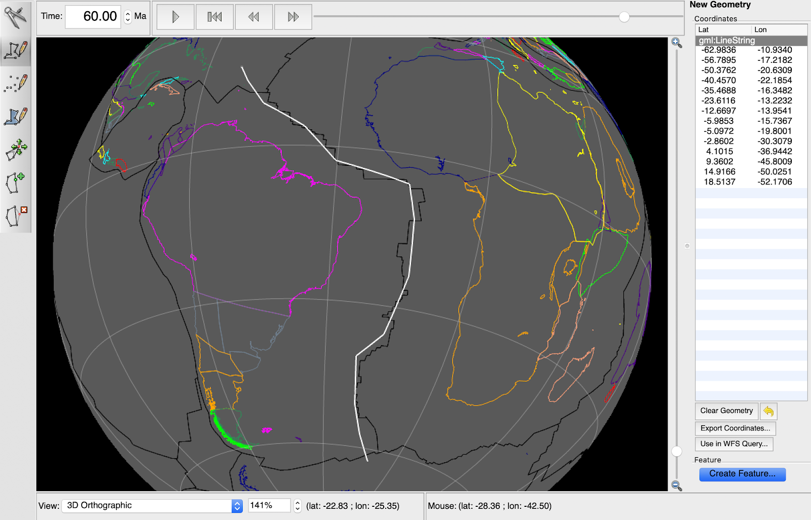
Figure 11. Digitise the new MOR to intersect the plate boundaries of the SAM or African plate.
- Click ‘Create Feature’ to open up the Create Feature window. Select ‘MidOceanRidge’ as the feature type and specify all properties as before (i.e., Left and Right plate IDs of 201 and 701 respectively, the Begin and End time to 60 and 20 Ma, respectively, and a new feature name) and click Next, and again Next (Figure 12).
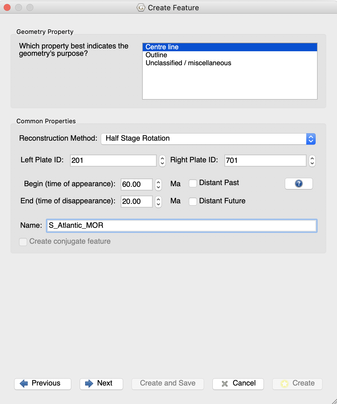
Figure 12. Specify all the properties of the new MOR feature in the ‘Create Feature’ window.
- As in Exercise 1, select the plate boundaries dataset to save your new MOR to, and click Create. You will then be taken back to the main GPlates window where you can reconstruct back to 20 Ma to check whether your MOR is reconstructing correctly.
Ideally, the endpoints of your MOR should continue to intersect the adjacent plate boundaries but in the situation in which they do not (Figure 13), refer to the Appendix before continuing.
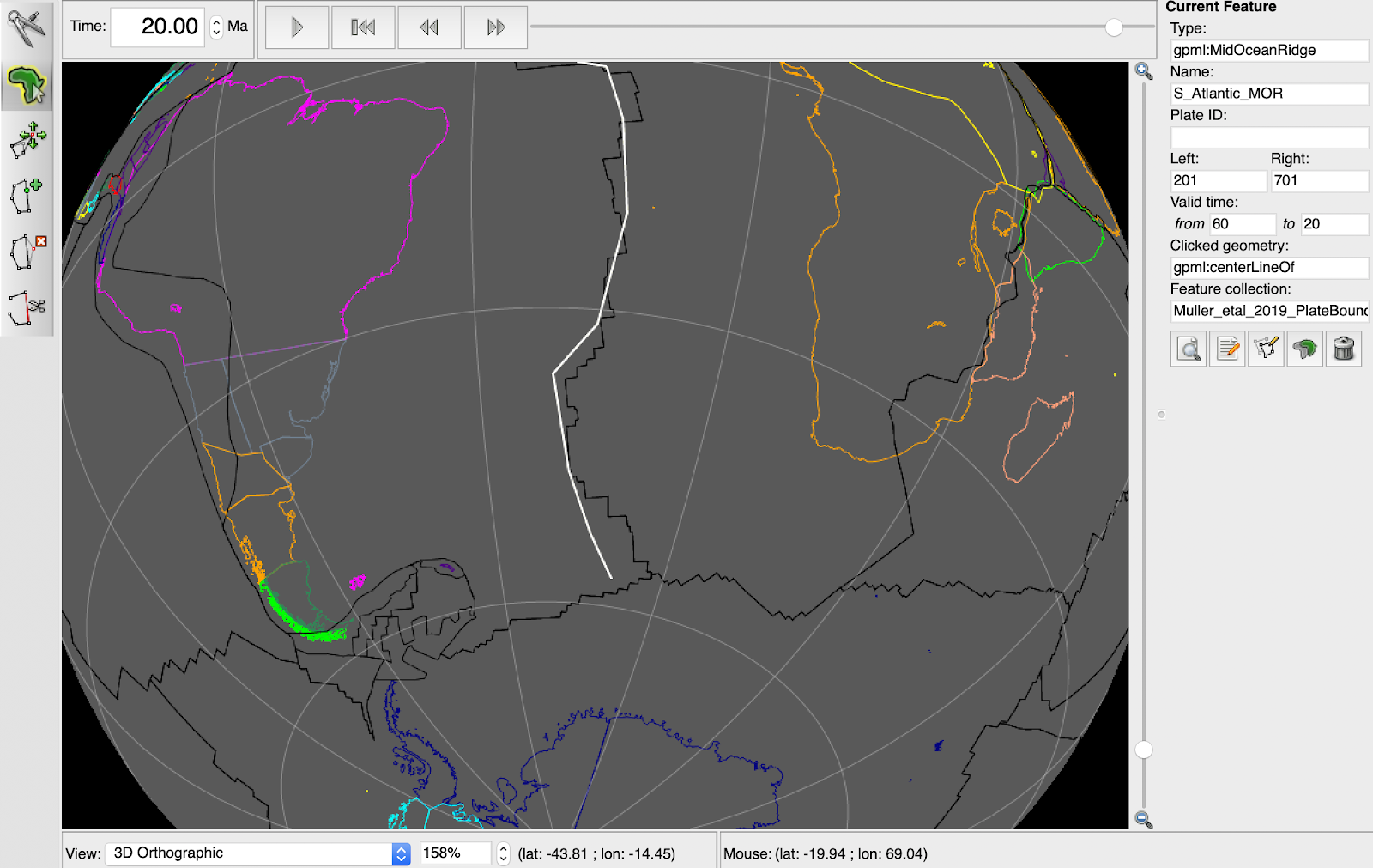
Figure 13. In this case, the southern end of the new MOR feature reconstructed at 20 Ma (circled) does not intersect with the pre-existing plate boundaries, and therefore must be modified.
Return to 60 Ma for the next steps.
- Under the Topology tab , use the ‘Select Feature’ tool to select the first plate polygon to be edited (we will choose the SAM Plate), and then select ‘Edit Topology Sections’ (Figure 14).

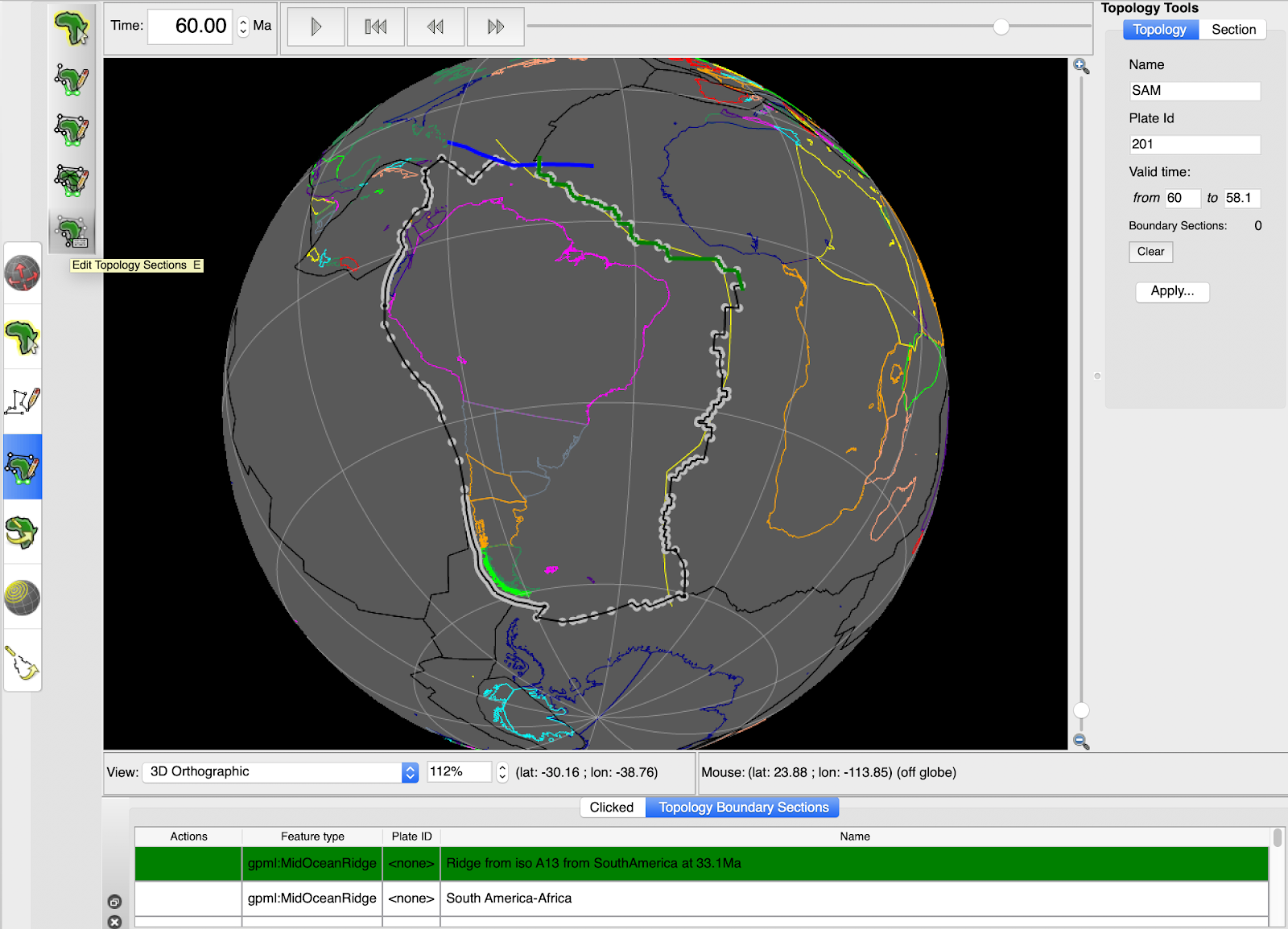
Figure 14. Under the ‘Topology’ icon, select the SAM Plate using the ‘Choose Feature’ tool and then select the ‘Edit Topology Sections’ tool.
- Click the problematic boundary that needs to be replaced. In this example, there are three sections to be removed: “Ridge from iso A13…”, “South America-Africa”, and “Malvinas Ridge Jump”. When you click on a boundary section, it will be highlighted in the Topology Sections list at the bottom of the GPlates window. Click the “X” button next to each of these boundary sections to remove them.
At this stage, the boundary topology should look like Figure 15. Notice that a “rubber-banding” artefact will appear until you insert the new MOR boundary.
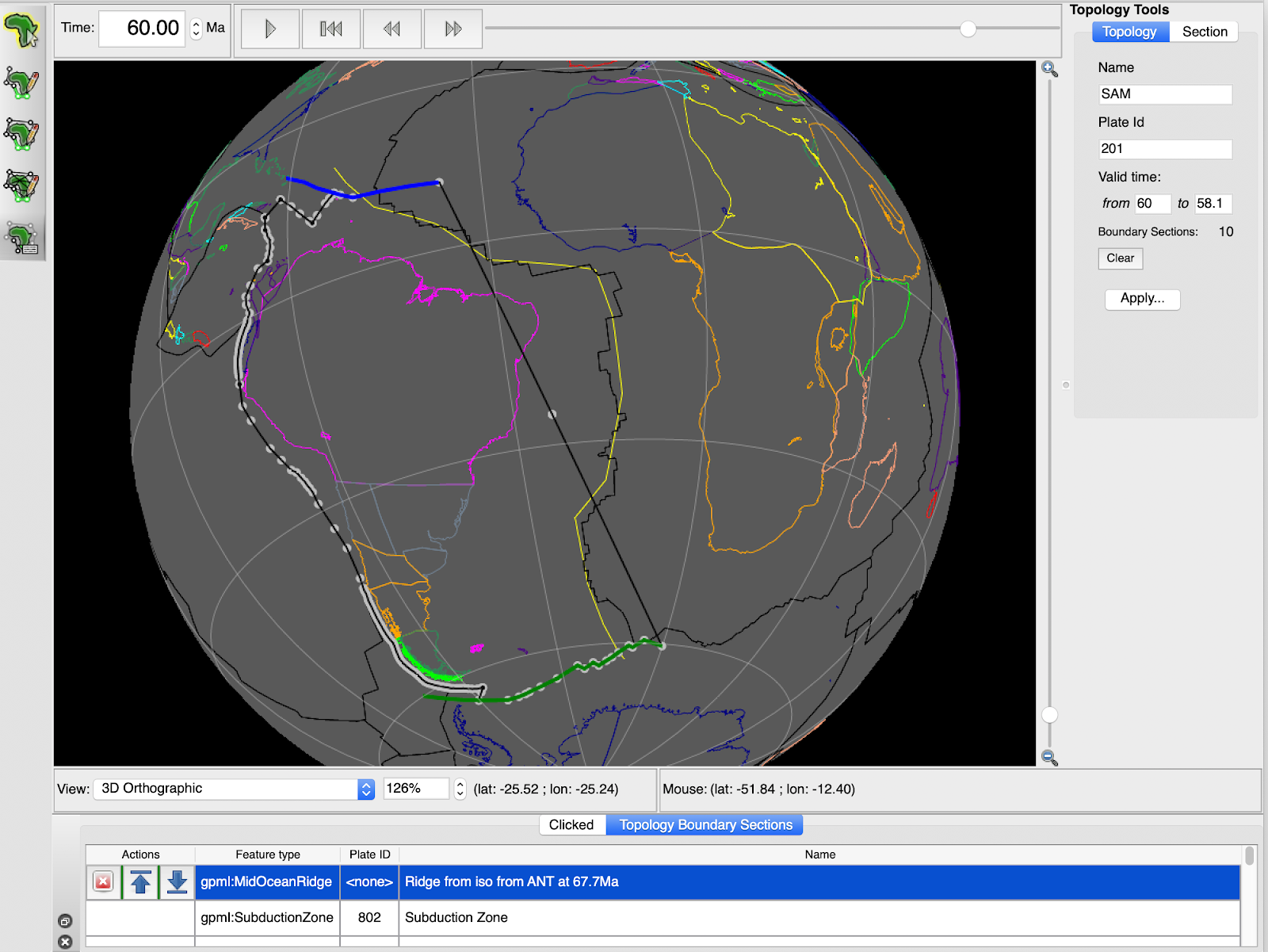
Figure 15. The SAM plate after removing the three pre-existing plate boundary segments.
- Select the new MOR feature by clicking on it, and then click the ‘Add’ button on the right-hand-side of the main window (Figure 16).
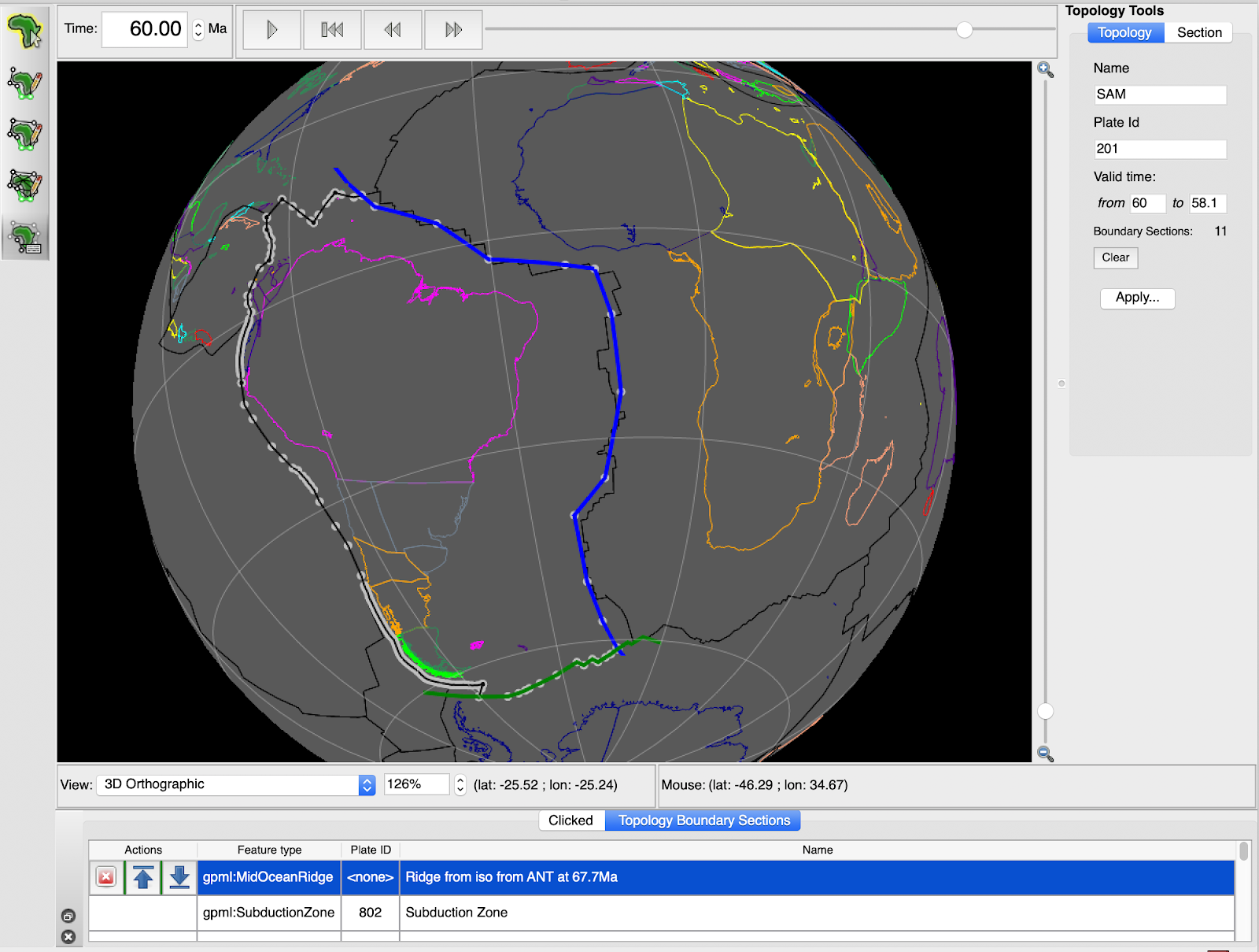
Figure 16. The SAM plate boundary topology after adding the new MOR boundary section.
In the Topology Tools window on the right-hand side of the main window, notice that the ‘Valid time’ for which the topology can exist for is limited from 60.1 to 58.1 (Figure 17). This is because the plate topology you are modifying will cease at 58.1 Ma (and transform into a ‘new’ one). The new MOR topology you have just incorporated into the polygon will similarly cease to exist at this point in time. If you select any feature, you will notice that the right-hand-side window will display the Valid time for which the feature will exist.
- Click Apply.
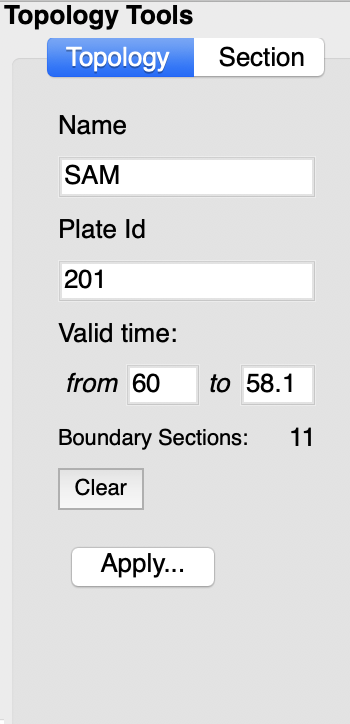
Figure 17. The ‘Valid time’ for which the newly edited topology can exist for is limited by the existing ‘Valid time’ of the old topology.
You have now successfully fixed one plate boundary topology.
- You must repeat this process on the other plate (in this case, the Africa plate) that shared the old MOR boundary.
Once you have done this you will want to make sure that you have not created any artefacts or discontinuities. The best way to see gaps, overlaps and rubber-banding artefacts is by turning off the lines and just displaying the resolved topologies.
- In the ‘Layers’ window, disable the green plate boundaries Reconstructed Geometries layer.
You can help to minimise these sorts of artefacts by carefully extending the new MORs to intersect at the same place as the old boundary (see Appendix). Nonetheless, there is usually a lot of manual work involved in introducing new MORs into existing plate boundary datasets.
References
Müller, R. D., Zahirovic, S., Williams, S. E., Cannon, J., Seton, M., Bower, D. J., Tetley, M. G., Heine, C., Le Breton, E., Liu, S., Russell, S. H. J., Yang, T., Leonard, J., and Gurnis, M., 2019, A Global Plate Model Including Lithospheric Deformation Along Major Rifts and Orogens Since the Triassic: Tectonics, v. 38, no. 6, p. 1884-1907. doi: 10.1029/2018tc005462
Appendix
Extending a new MOR to intersect with existing plate boundaries
If intending to replace an existing MOR with a new MOR feature, it is crucial that the new MOR geometry intersects with pre-existing plate boundaries in order for the user to edit the new topology in. If the MOR fails to intersect these plate boundaries, which may be the case after reconstructing back through time, it is possible to interactively extend the MOR to intersect with the required plate boundaries.
Using the ‘Choose Feature’ tool, select the problematic MOR and click the ‘Insert Vertex’ tool (Figure 18).
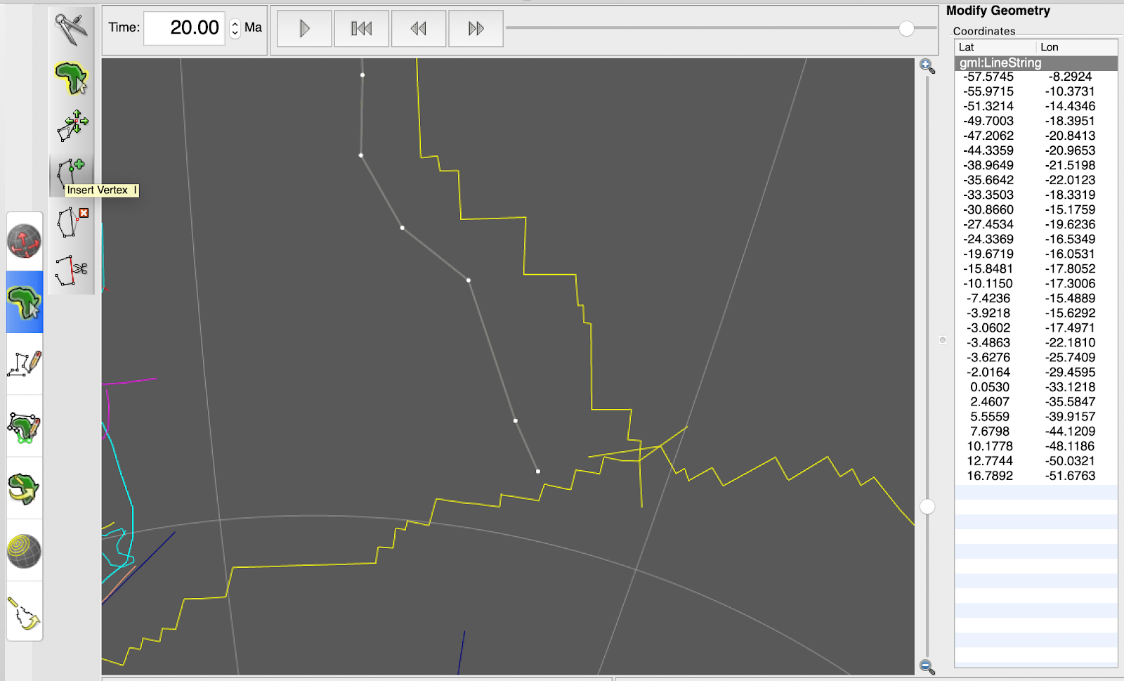
Figure 18: Select the MOR feature and click the ‘Insert Vertex’ tool.
Add points to make the sure MOR intersects with neighbouring boundaries (Figure 19).
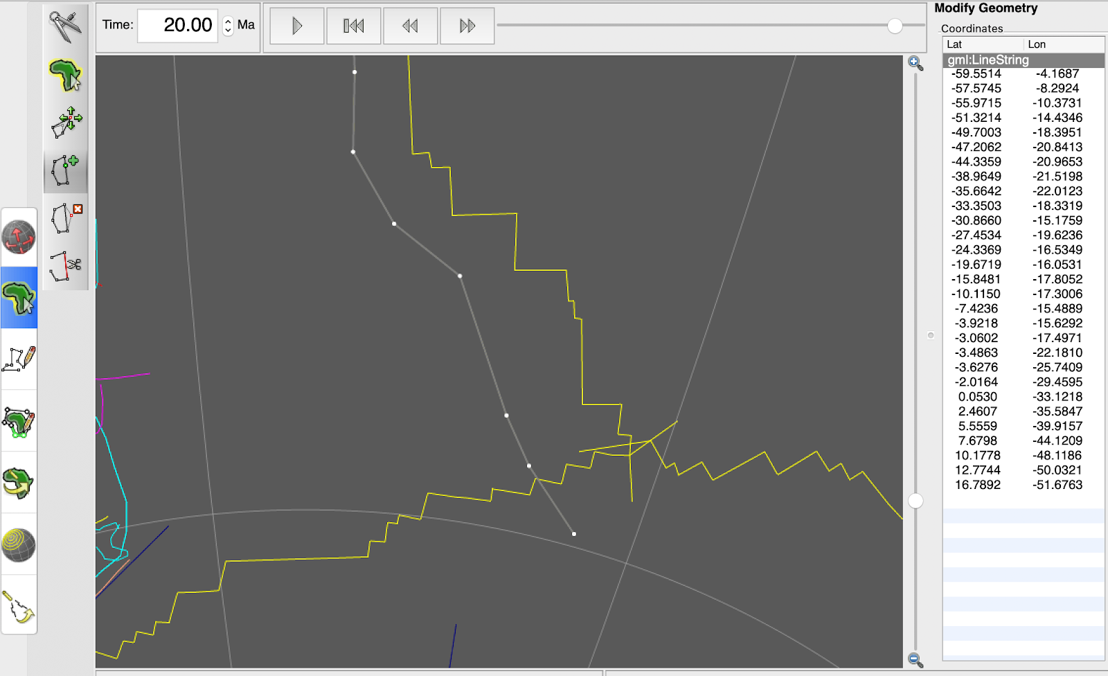
Figure 19: Plot points interactively to extend the MOR until it intersects with adjacent plate boundaries.
Once you are satisfied, select any other tool on the main interface (such as the ‘Choose Feature’ tool) to halt the process. You have now successfully extended your MOR feature!