Georeferencing Images for use in GPlates

Authors: Serena Yeung

It has been updated by Behnam Sadeghi, using the latest Muller et al. (2019) plate reconstructions and GPlates 2.2 interface!

EarthByte Research Group, School of Geosciences, The University of Sydney, Australia

Aim

Background

Included data

Exercise 1 – Georeferencing the Lord Howe Rise and importing it into GPlates

Exercise 2 – Georeferencing East Antarctica using a polar projection and importing it into GPlates

References

Aim

This tutorial aims to teach the user how to (1) georeference an image from a paper using ArcGIS 10.1, (2) import the georeferenced image into GPlates and (3) know how to deal with images which do not suit geographic coordinate systems, such as polar areas.

Background

Georeferencing involves using geographic map coordinates to assign a spatial location to a map feature such as an image from a scientific paper. GPlates can import a georeferenced image as a raster and correctly place it on the globe and its coastlines, provided that we include the extent of the raster in degrees (latitude and longitude). This is simple to obtain if the map layer you are georeferencing to use a geographic coordinate system which employs latitude and longitude such as WGS 1984.

It becomes particularly problematic however if you wish to georeference an image which better suits a projected coordinate system, as these do not employ latitude and longitude. This is the case when working with images located in extreme latitudes such as in polar areas. It is very difficult trying to georeference a map of Antarctica if the base map layer is not in a polar projection, causing the poles to be compressed, elongated and very hard to match up to.

This tutorial focuses on how to produce georeferenced images in ArcGIS 10.1 which meet the requirements of being able to be imported into GPlates as a raster. Note that other versions of ArcGIS should also work. This tutorial will also run through how to deal with map projections which do not employ latitudes and longitudes. This tutorial is not designed to teach users how to georeference images in ArcGIS, and assumes a basic knowledge of how to do so. If you require instructions on how to georeference, refer to this YouTube tutorial <http://www.youtube.com/watch?v=PHtxbpboDro> or this ArcGIS webpage <http://help.arcgis.com/en/arcgisdesktop/10.0/help/index.html#//009t000000mq000000>

Included data

Click here to download the data bundle for this tutorial.

This tutorial includes a dataset comprised of two separate folders:

(1) files for the ArcGIS portion of the tutorial

GoodgeFinnAeromagneticsAntarctica.png

NorvickLordHoweRise.png

Muller_etal_2019_Global_Coastlines.shp

(2) files for the GPlates portion of the tutorial

Muller_etal_2019_Global_StaticPlatePolygons.gpmlz

Muller_etal_2019_CombinedRotations.rot

Muller_etal_2019_Global_Coastlines.gpmlz

This tutorial dataset is compatible with GPlates 2.2.

Exercise 1 – Georeferencing the Lord Howe Rise and importing it into GPlates

Any raster image can be georeferenced. When obtaining figures from papers, you can either save an image of the figure directly, or take a screenshot and use an image editing program to save it.

In this exercise we will georeference a PNG image of the Lord Howe Rise (Norvick, 2008) which is included in the tutorial dataset (NovickLordHoweRise.png).

But firstly, load the Muller et al. 2019 Coastlines shapefile (Muller_etal_2019_Global_Coastlines.shp) into ArcMap using the ‘Add Data’ button.

This coastlines shapefile will be used to check the alignment of our image once we begin to georeference it.

Note that the coastlines should not be used as the basis for georeferencing your image. They should only be used in this way if the number of known latitudes and longitudes provided in the original raster image are of an insufficient number. That is, where possible, always ‘Input DMS of Lon and Lat’ when creating control points, rather than matching control points to coastlines.

Change the symbology of the Muller et al Coastline layer in the Properties window so that the outline is black and a width of 2.0 for ease in distinguishing between the Coastline and the raster image to be georeferenced.

Then, load the raster image ‘NovickLordHoweRise.png’ into ArcMap.

Use the Georeferencing toolbar to start adding control points to the non-georeferenced Lord Howe Rise layer. Input the DMS of latitude and longitude of each control point. Refer to the coastlines to check how accurate your georeferencing is.

You may need to match some control points to the coastlines if you do not have enough.

You may also need to transform the layer so that it better fits the coastlines. Try using a 2nd order polynomial transformation.

If you are unsure of how to do these georeferencing steps in ArcGIS, refer to this YouTube tutorial <http://www.youtube.com/watch?v=PHtxbpboDro>

Your final image should look something like this (Figure 1):

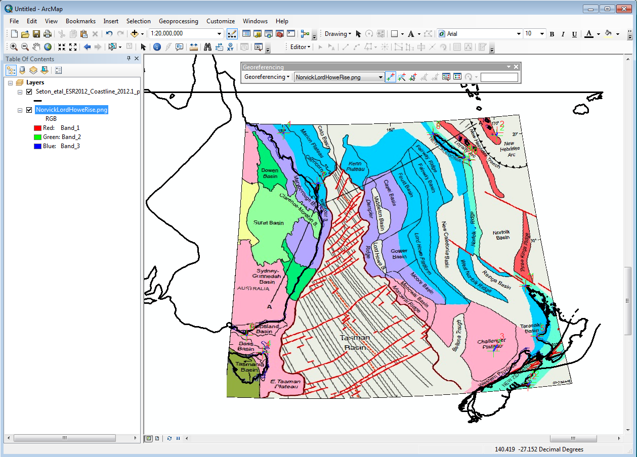
Figure 1. Georeferenced image of the Lord Howe Rise, transformed using a 2nd order polynomial. Coastline file is in black.

Rectify the image and save it as a TIFF file. While not necessary, specify the Resample Type as Bilinear Interpolation (for continuous data). You may also wish to add ‘_rectify’ to the end of the filename (NovickLordHoweRise_rectify) to differentiate it from the original non-georeferenced image layer.

Change the value of the ‘NoData as’ field from 256 to 0. If left as 256, ArcGIS will export the image as a black box.

Specify the output location and click Save (Figure 2).

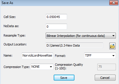
Figure 2. Rectify the image of the Lord Howe Rise. In the Save As window, specify the resample type, filename and export format, then click Save.

(Note: The format box appears grey when the ‘Save As’ window is opened. In order to change the format to a TIFF file, we need to specify the ‘Output Location’. Click on the folder icon next to ‘Output Location’, and highlight the folder we would like to save the new georeferenced file in. Then click ‘Add’, and this should allow us to specify the correct format.)

We can now import the rectified, georeferenced image as a raster into GPlates. In order to complete the import stage, however, GPlates requires the Extent of the raster in degrees (latitude and longitude).

In order to obtain this information, load the rectified, georeferenced TIFF image into ArcGIS using the ‘Add Data’ button. Right click on the georeferenced layer (NovickLordHoweRise_rectify) and select Properties. Click on the ‘Source’ tab and scroll down to the heading ‘Extent’, where you will find Top, Left, Right and Bottom coordinates in degrees (Figure 3). These are the coordinates we will enter straight into GPlates.

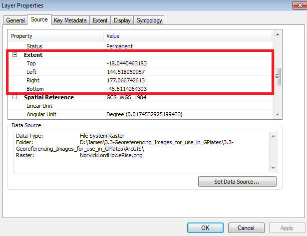
Figure 3. Latitudinal and longitudinal extent of the georeferenced Lord Howe Rise raster, viewed under the Source tab in the Layer Properties window.

Open GPlates and load the following included Coastline, Static Plate Polygon and rotation files using ‘Open Feature Collection’ (Figure 4).

Muller_etal_2019_Global_Coastlines.gpmlz

Muller_etal_2019_Global_StaticPlatePolygons.gpmlz

Muller_etal_2019_CombinedRotations.rot

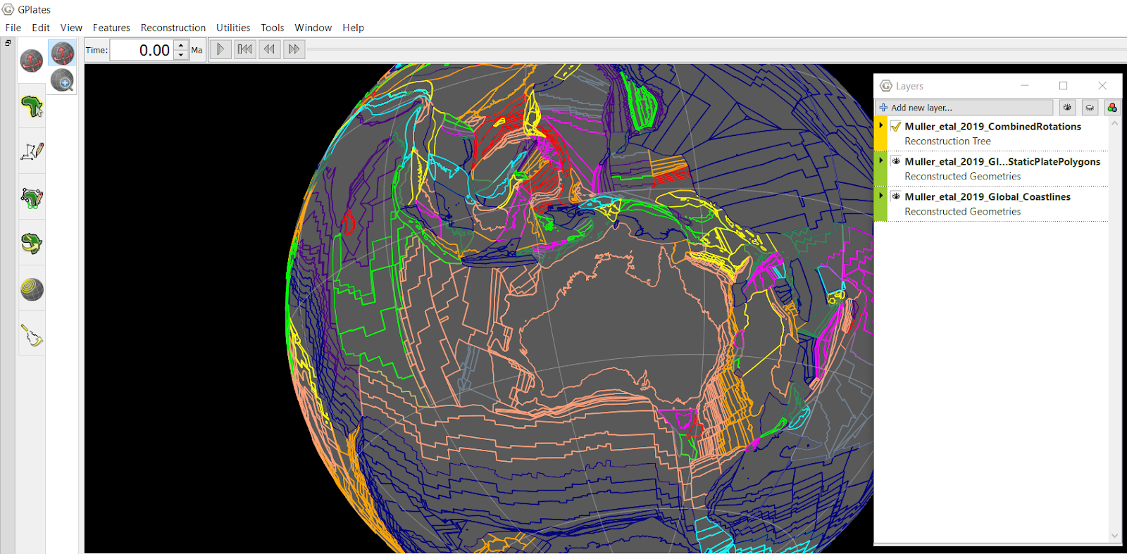
Figure 4. GPlates with the Muller et al coastlines, Earthbyte Static Plate Polygons and the Muller et al rotation file loaded.

We will now load the georeferenced image (NovickLordHoweRise_rectify) into GPlates as a raster file. Select 'File', 'Import', and 'Import Raster'.

Navigate to where your image is saved, select the image and click 'Open'.

In the first Import Raster window, leave the band name as the default (band_1) and click Next.

In the second Import Raster window, under Georeferencing, you are prompted to specify the location of the raster. Switch back to ArcGIS where you have the Properties window open and transfer the Top, Left, Right and Bottom coordinates straight into GPlates (Figure 5). Click Next.

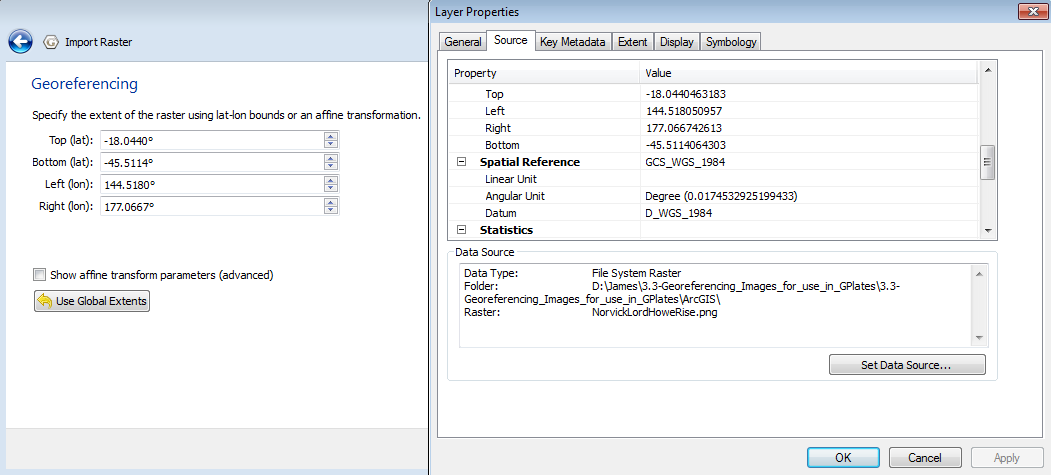
Figure 5. Enter in the coordinates specified in the Extent of the raster in ArcGIS straight into the Georeferencing window in GPlates, ensuring that Top, Left, Right and Bottom are in the correct order.

In the third Import Raster window, under Feature collection, keep the default < Create a new feature collection > option and click Finish.

You will now see your raster placed correctly on the globe. Centre the view on eastern Australia and New Zealand and you should see your image. Notice how the coastlines of the Muller et al model match the coastlines of your image. To see the matching coastlines more clearly, change the colour of the Muller et al coastlines to black using ‘Manage Colouring’.

Note: if the image appears black in GPlates, or the colour appears odd, check the folder in which your rectified image was saved. If it is black/oddly coloured too, this means that ArcGIS exported the rectified image incorrectly. Ensure that the value of the ‘NoData as’ field in the Rectify window is 0, not 256. If left as 256, ArcGIS will export the image as a ‘black box’.

If this fails to work, you may have to experiment with different output types when rectifying your image in ArcGIS (e.g., TIFF, JPG). We have found that georeferencing a GIF and then rectifying it as PNG works. Import the image as a raster in GPlates as specified above, and you should see your image displayed correctly (Figure 6).

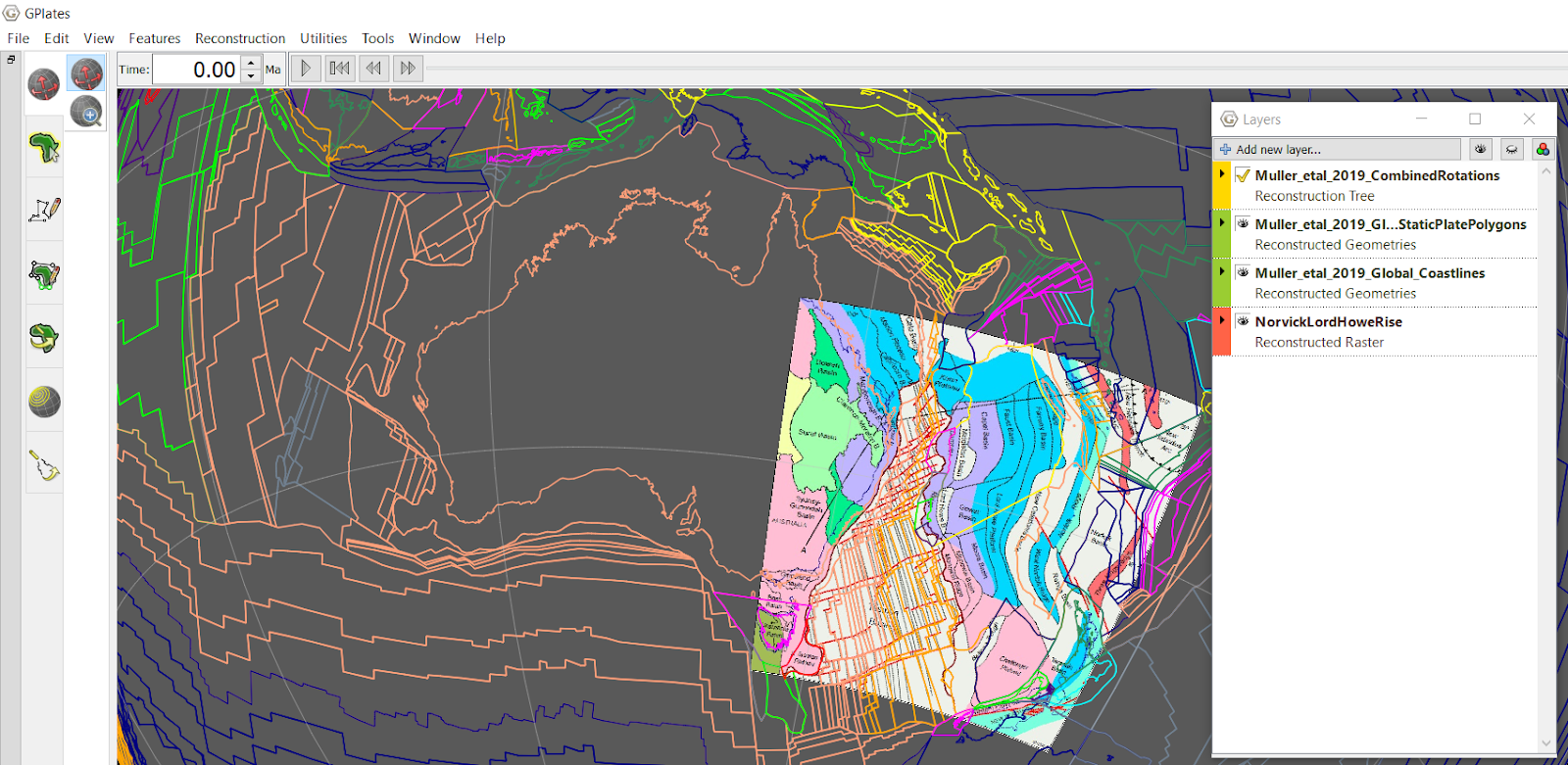
Figure 6. Load the raster of the Lord Howe Rise into GPlates and you will see your georeferenced image placed correctly on the globe. To see the matching coastlines more clearly, change the colour of the Muller et al coastlines to black using ‘Manage Colouring’.

We will now connect the georeferenced image to the static plate polygon file. This allows the image to reconstruct correctly through time. Notice that if you try reconstructing to say 20 Ma, the image stays put relative to the movement of the plates.

To connect the image to the plate polygons, expand the raster file in the Layers window by clicking on the triangle beside the file name. Under 'Reconstructed polygons:', click 'Add new connection' and select the static polygon file (Muller_etal_2019_Global_StaticPlatePolygons.gpmlz) (Figure 7).

Figure 7. In order for the Lord Howe Rise raster to reconstruct correctly through time, connect the Lord Howe Rise raster to the Muller et al Static Polygons in the Layers window by clicking ‘Add new connection’.

Notice that now if you reconstruct through time, such as to 20 Ma, the raster will stay attached to the plate polygons (Figure 8).

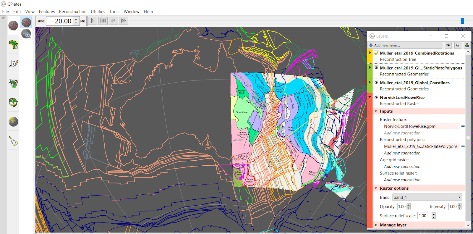
Figure 8. Once the raster is connected to the static plate polygons, the Lord Howe Rise raster will stay attached to the plate polygons when you reconstruct through time, such as to 20 Ma.

You have now learnt how to georeference images in ArcGIS for use in GPlates!

Exercise 2 – Georeferencing East Antarctica using a polar projection and importing it into GPlates

When georeferencing images located in the extreme latitudes such as polar areas, it is much easier to use a projected coordinate system rather than a geographic coordinate system. Geographic coordinate systems such as WGS 1984 tend to compress and elongate the poles, making it very difficult to visualise and add control points.

To prepare a georeferenced image that can be imported straight into GPlates, we must ensure that the georeferenced image is saved in a format which uses latitude and longitude. Hence, the best way to go about this is to georeference the image using a polar stereographic projection, but prior to rectifying the image, the projection should be changed back to WGS 1984 to ensure the output is in latitude and longitude.

To do this, load the image to be georeferenced into ArcGIS using the ‘Add Data’ button. In this exercise we will georeference a PNG image of East Antarctica (Goodge and Finn, 2010) which is included in the tutorial dataset (GoodgeFinnAeromagneticsAntarctica).

Change the dataframe's coordinate system by right-clicking 'Layers' in the Table Of Contents window and selecting 'Properties' (Figure 8).

Figure 8. In order to reference an image using a different coordinate system, right click ‘Layers’ in the Table of Contents, and select ‘Properties’.

This will open the Data Frame Properties window. Under the 'Coordinate System' tab, scroll down and expand the 'Projected Coordinate Systems' folder, expand the 'Polar' folder and select 'WGS 1984 Antarctic Polar Stereographic'. Click OK (Figure 9).

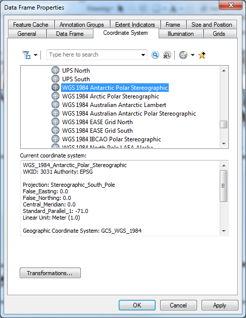
Figure 9. Select the WGS 1984 Antarctic Polar Stereographic projection system in the Data Frame Properties window, then press OK.

You will now be able to see Antarctica much more clearly in this polar projection. Start to georeference the image by adding control points as before using the Georeferencing toolbar (Figure 10).

In this circumstance, you will mostly likely need to match all control points to the coastline file. There will not be enough control points to ‘Input DMS of Lon and Lat’.

You may not find it necessary to transform it from a 1st Order Polynomial to a 2nd Order Polynomial. Once you have finished georeferencing, click ‘Update Georeferencing’ in the drop-down menu of your Georeferencing toolbar.

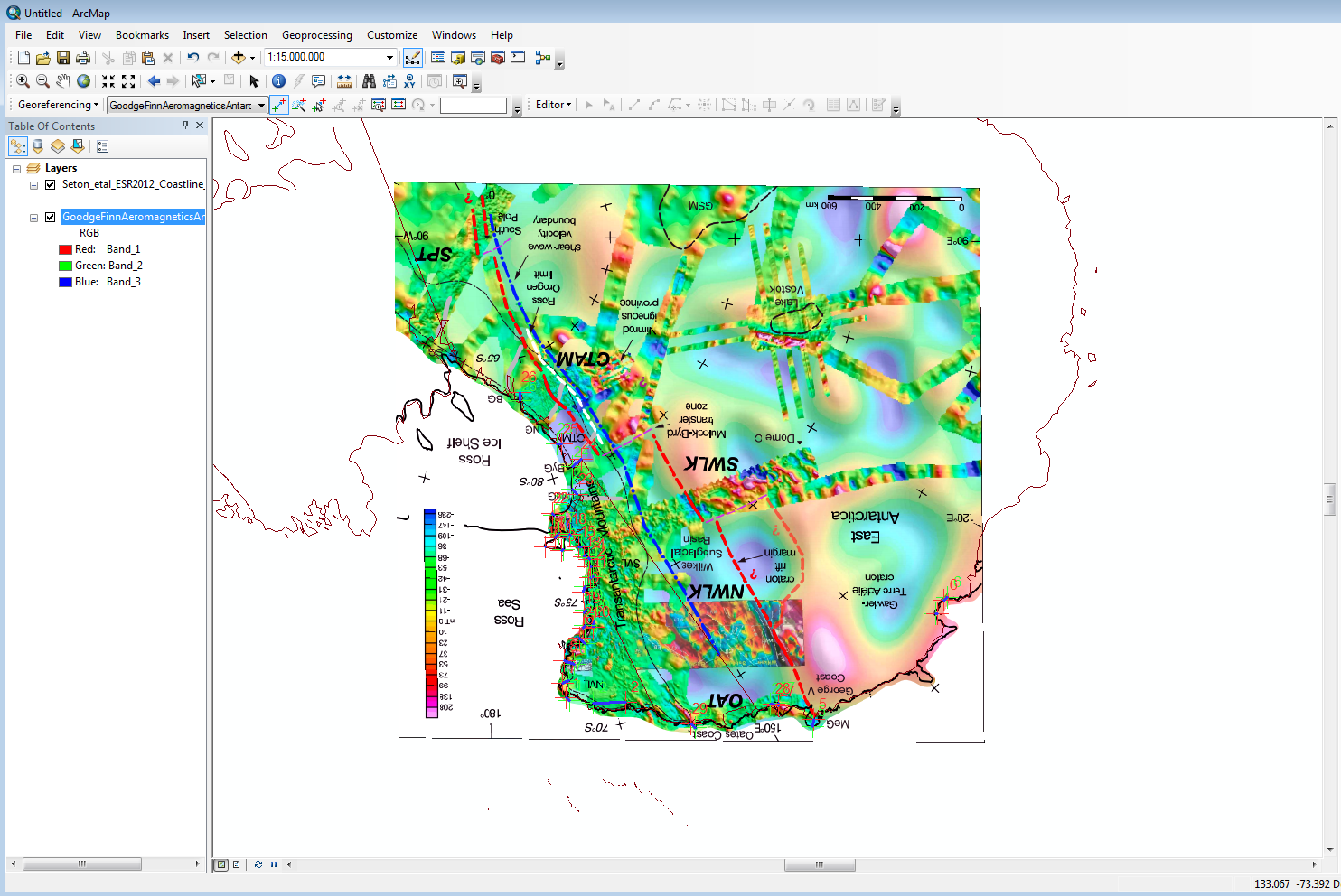
Figure 10. Add control points in order to georeference the of Antarctica onto the map coordinates of the Muller et al coastlines.

Change the data frame’s coordinate system back to the global coordinate system WGS 1984 by right clicking ‘Layers’ and selecting ‘Properties’. Scroll down and expand the last folder named ‘Layers’ and select ‘GCS_WGS_1984’. Click OK (Figure 11).

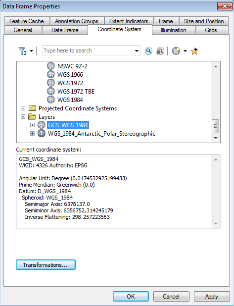
Figure 11. Change the data frame’s coordinate system back to WGS 1984 in the Data Frame Properties window, which can be opened by right clicking ‘Layers’ in the Table of Contents window and selecting ‘Properties’.

Your georeferenced image of Antarctica should look stretched out, but be in the correct spot (Figure 12).

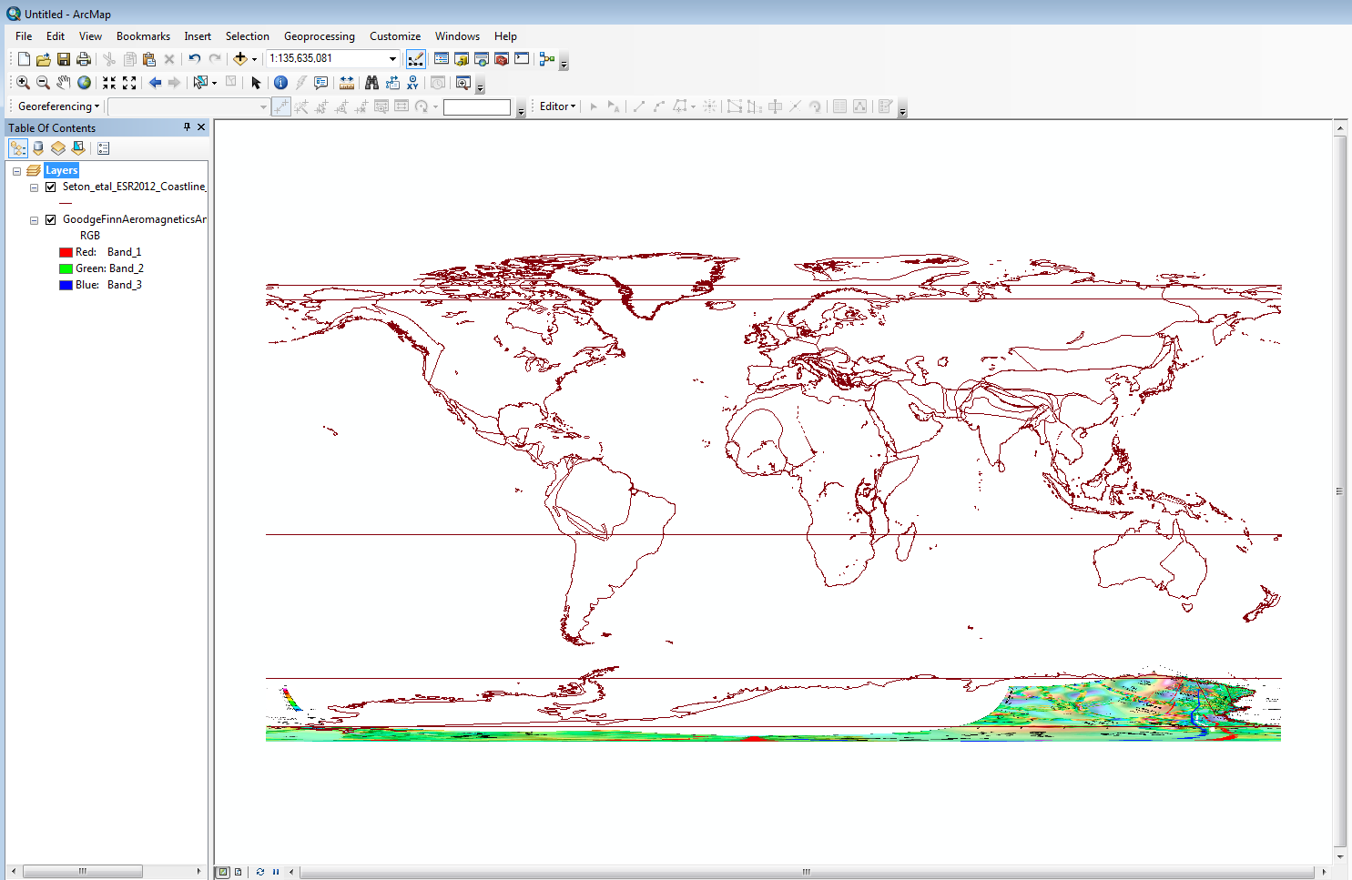
Figure 12. The georeferenced image of East Antarctica projected using the geographic coordinate system WGS 1984.

If your image of Antarctica turned into a block colour and is stretched out over the entire frame of your GCS WGS 1984 projection, this means that you did not ‘Update Georeferencing’ while in the Antarctic Polar Stereographic projection. Return to the Polar projection, click ‘Update Georeferencing’ under the drop-down ‘Georeferencing’ button, then return to the Geographic coordinate system.

Unlike the previous example, we cannot ‘Rectify’ the image of Antarctica when it is displayed in a projection other than the one it was originally georeferenced to. Since we require latitude and longitude in the Geographic coordinate system, this becomes a problem.

One alternative way is to export the image as a raster.

Right click the Antarctic image layer in the Table Of Contents window, and under ‘Data’, select ‘Export Data…’ (Figure 13).

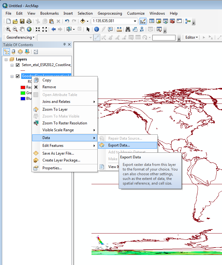
Figure 13. Export your georeferenced image as a raster by right clicking the layer, and under Data select ‘Export Data’.

In the Export Raster Data window which opens, change the Spatial Reference to ‘Data Frame (Current)’. Notice that the Extent in the attribute table will change accordingly.

Select a suitable Location to save to by clicking the folder button, specify the name (e.g., GoodgeFinnAeromagneticsAntarctica_WGS1984) and change the format to PNG.

Change the value of the ‘NoData as’ field from 252 to 0. If left as 252, ArcGIS will export the image as a ‘black box’.

Click Save (Figure 14).

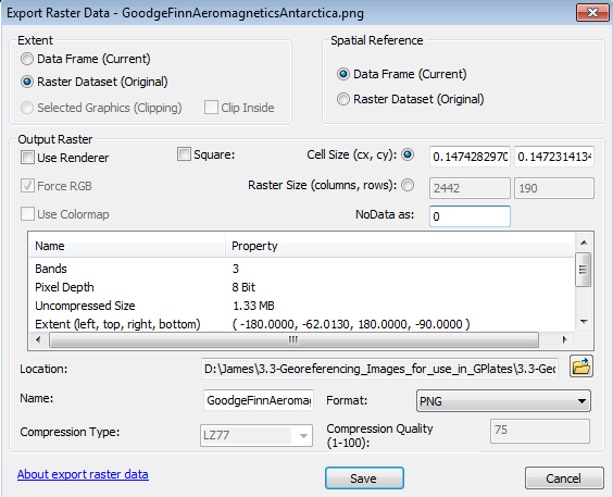
Figure 14. In the Export Raster Data window, change the Spatial Reference to ‘Data Frame (Current)’. Specify a file location, name and format, then click Save.

Load your newly exported data into ArcGIS by using the ‘Add Data’ button. Right click the layer, select Properties, and scroll down to the ‘Extent’ and ‘Spatial Reference’ information. Notice that the spatial reference is now GCS_WGS_1984 and not the polar projection, and that the extent is in latitude and longitude (Figure 15).

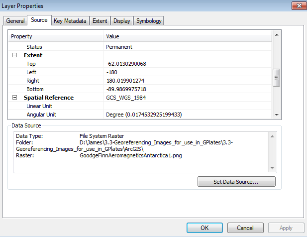
Figure 15. Latitudinal and longitudinal extent of the georeferenced East Antarctica raster, viewed under the Source tab in the Layer Properties window.

You are now ready to load the image into GPlates!

Open GPlates and load the following included Coastline, Static Plate Polygon and rotation files using ‘Open Feature Collection’ if you haven’t already.

Muller_etal_2019_Global_Coastlines.gpmlz

Muller_etal_2019_Global_StaticPlatePolygons.gpmlz

Muller_etal_2019_CombinedRotations.rot

We will now load the georeferenced image (GoodgeFinnAeromagneticsAntarctica_WGS1984) into GPlates as a raster file. Select 'File', 'Import', and 'Import Raster'. Navigate to where your image is saved, select the image and click 'Open'.

Import the raster as you did using the Lord Howe Rise example. If you are prompted to specify an age of the raster in the first import window, type 0 (0 Ma). In the next few windows, keep all defaults except the georeferencing coordinates. Type in the latitudes and longitudes of your Antarctic image straight from the ‘Extent’ section in your Layer Properties box from ArcGIS (Figure 16).

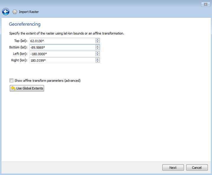
Figure 16. Use ‘Import Raster’ to import the georeferenced East Antarctica raster into GPlates. Enter in the coordinates specified in the Extent of the raster in ArcGIS into the GPlates Georeferencing window.

Create a new feature collection and click ‘Create’.

Centre your globe on Antarctica and you should see your image in the correct location (Figure 17). Ensure that the reconstruction time is reset to 0 Ma from the previous exercise.

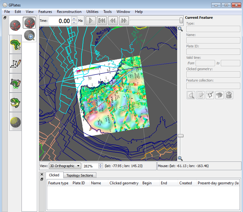
Figure 17. Your imported georeferenced raster of East Antarctica should be placed correctly on the globe. Ensure that the reconstruction time is reset to 0 Ma from the previous exercise.

Note once more: if the image appears black in GPlates, or the image appears odd in colour, ArcGIS exports the rectified image incorrectly. Change the value of the ‘NoData as’ field in the Rectify window from 252 to 0. If this fails to work, georeferencing a GIF and then exporting it as PNG works. Import the image as a raster in GPlates as specified above, and you should see your image displayed correctly.

Connect the Antarctic image to the static plate polygons in GPlates as you did in the previous exercise. Expand the raster file in the Layers window by clicking on the triangle beside the file name. Under 'Reconstructed polygons:', click 'Add new connection' and select the static polygon file (Muller_etal_2019_Global_StaticPlatePolygons).

Notice that now if you reconstruct through time, the raster will stay attached to the plate polygons.

You have now learnt how to georeference polar images in ArcGIS for use in GPlates!

References

Goodge, J.W. and Finn, C.A. 2010. Glimpses of East Antarctica: Aeromagnetic and satellite magnetic view from the central Transantarctic Mountains of East Antarctica. Journal of Geophysical Research 115

Norvick, M.S., Langford, R.P., Hashimoto, T., Rollet, N., Higgins, K.L. and Morse, M.P. 2008. New insights into the evolution of the Lord Howe Rise (Capel and Faust basins), offshore eastern Australia, from terrane and geophysical data analysis. In: Eastern Australasian Basins Symposium III: Energy security for the 21st century, Blevin, J.E., Bradshaw, B.E. and Uruski, C. eds. Petroleum Exploration Society of Australia Special Publication: 291–310

Müller, R. D., Zahirovic, S., Williams, S. E., Cannon, J., Seton, M., Bower, D. J., Tetley, M. G., Heine, C., Le Breton, E., Liu, S., Russell, S. H. J., Yang, T., Leonard, J., and Gurnis, M., 2019, A Global Plate Model Including Lithospheric Deformation Along Major Rifts and Orogens Since the Triassic: Tectonics, v. 38, no. 6, p. 1884-1907. doi: 10.1029/2018tc005462.